チュートリアル：細胞画像を使った初めてのディープラーニング

ディープラーニング完全に理解した
Python経験ほぼほぼゼロから始める細胞画像のディープラーニング
version 1, 5/15/2020
高尾大輔
東京大学大学院医学系研究科

近年のAI技術の急速な発展と普及の波は生命科学分野にも広がっています。
特に、ディープラーニングを含む機械学習はすでに多くの成果を挙げています。
そろそろ自分の研究にもAI技術を取り入れてみたい！…けど何から始めたらいいか分からない！
という方も多いのではないでしょうか？
このチュートリアルでは、実際に顕微鏡画像とディープラーニングを使って細胞周期を分類する
Pythonコードを動かしてみます。
想定しているレベルは、Pythonを触ったことぐらいはあるという程度の初心者です。
難しいことは考えずにとりあえずサンプルコードとデータを使って動かせるようにしています。
使用するコードとデータは最近発表した論文で使われたものなので、実用性も十分あります。
筆頭著者である学部学生（研究当時）の長尾さんが作ってくれたコードに多少手を加えたものを
GitHubに公開しています。
プログラミングほぼ未経験の学生が数カ月の間にこれほどのコードを作れるようになりました。
これは初心者にとっては励みとなる事例ではないでしょうか。
近くに適切な指導者がいないと少しハードルは上がるかもしれませんが、上記の通り超初心者でも
動かせるようにしたつもりです。
細胞画像の分類という例題に挑戦するわけですが、できれば事前に論文に目を通してざっと内容を
理解しておいてもらえるとスムーズです（流れを理解する程度で大丈夫です）。
日本語の解説も書いたので参考にしてください。
論文
https://www.molbiolcell.org/doi/10.1091/mbc.E20-03-0187
解説
https://daisuketakao.wixsite.com/labwork/post/細胞画像のわずかな特徴の違いの見分け方をaiに教えてもらおう

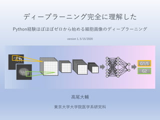
目標
蛍光染色した培養細胞の顕微鏡画像から細胞周期を判定します。
ここではG2期のマーカーであるCENP-Fを使って、間期の細胞をG2とG1/S（notG2と表記）に
あらかじめ分類したデータセットを使います。
論文ではこのマーカーを使わずにG2とnotG2を分類する機械学習モデルを開発しました。
実際にDNA (Hoechst)やゴルジ体(GM130)の染色画像からG2とnotG2を分類してみましょう。
方法
ディープラーニングの一種である畳み込みニューラルネットワーク(CNN)を使います。
公開されているPythonコードはJupyter Labで使用する前提で書かれています。
CNN用のフレームワークにはKerasを使用しています。
仮想環境を構築してパッケージのバージョンを指定して……いきなりハードル高いです笑
なるべく難しいことは抜きにとにかくまずは気軽に動かしてみよう！というのが今回の重要な
コンセプトなので、Google Colabを使用することにしました。
仮想環境を構築してJupyter Labで実行する場合は論文のパッケージバージョン情報を参照してください。
必要なのはGoogleアカウントとインターネット環境だけです。有料ソフトは使いません。
環境整備の段階から始められるように順に説明していきますのでご安心ください。
元々Jupyter Labで作ったスクリプトなので、以降に説明するように少し書き換えが必要な箇所が
あります。
説明に従って基本的には順番にセルを実行していけばうまく動くはずです。
それではさっそく始めましょう。

0. ソースコードとサンプルデータの取得
実際のスクリプトファイルとサンプルデータを取得しておきます。
ほぼ生データに近い顕微鏡画像ファイルからスタートできるようになっています。
・ソースコードをGitHubからダウンロード。
・サンプルデータをZenodoからダウンロード。
・Google Colabのインストール。

ソースコードとデータのダウンロード
ソースコードは論文からリンクされているGitHubのリポジトリからダウンロードします。
https://github.com/dtakao-lab/Nagao2020
GitHubの操作にあまり馴染みがない場合、今回はとりあえず手動でダウンロードするのが一番
手っ取り早いです。
Codeフォルダ内にある4つの.ipynb形式のファイルがソースコードです。
画像データはここではチュートリアル用に用意したものをZenodoからダウンロードします。
https://doi.org/10.5281/zenodo.3825945
HeLa_Hoechst_GM130_CENP-F.zipがメインのデータです(188.6 MB)。
残りの4つは切り出された細胞画像です。詳しくはセクション1の最後で説明します。

GitHubの説明にもあるように、以下の階層構造（下図左）となるようにフォルダを作成してください。
このようなフォルダが存在している前提でスクリプトは書かれています。
class1とclass2はここではそれぞれG2とnotG2という名前にしてください。
例えばMy Drive>Colab Notebooks>CellCycleというフォルダを作ってそこをrootとします（下図右）。
全く同じにする必要はありませんが、同じ構造にしておくとこのチュートリアルを進めやすくなるかと
思います。
Zenodoからダウンロードした画像データもここにコピーしておいてください。
root
事前に自分で作成する
(imageフォルダ内には
サブフォルダも)
チュートリアル用の画像ファイル
（Zenodoからダウンロード）
GitHubから
ダウンロード

Google Colabを使えるようにインストールします。この操作は実際に使う時でもかまいません。
Google Drive内の適当なファイルを右クリックしてアプリを追加します。
アプリ一覧の中から”Colaboratory”で検索すると出てくるのでインストールします。
使い方はこのチュートリアルでも説明しますが、こちらのリンク先の説明が分かりやすいです。
https://www.codexa.net/how-to-use-google-colaboratory/
適当な場所を右クリック

1. 細胞画像の切り出しとデータセット作成
訓練データ（※）・テストデータ作成の下準備として、個々の細胞を切り出した画像を作成します。
※学習データ、教師データなどいろいろ呼び方がありますが、ここではコード内の”train”表記に合わせて訓練データと呼びます。
オリジナル画像には16-bitのTIFF形式で保存された顕微鏡画像を使います。
共焦点顕微鏡で取得したZスタック画像を最大値投影(MIP)した画像で、1枚あたりに概ね10–20程度の
細胞が含まれています。
・二値化した核の画像の重心を基準に指定サイズの正方形ROIで画像を切り出す。
・8-bitのBMPに変換
・CNNに渡す画像（ここではHoechst + GM130)とアノテーション用の画像（ここではCENP-F)を
分離する。
・アノテーション用の画像を指標にしてCNNに渡す画像を手作業で分類する（ここではG2とnotG2）。

まずGoogle Colabで”1_CropImage.ipynb”を開きます。こんな感じ。
見た目や操作感はJupyter Labとよく似ています。
Jupyter Labで作られたスクリプトなので、Google Colabで使えるように少し書き直します。
ちょっとしたお作法のようなものです。

from google.colab import drive
drive.mount('/content/drive')
一番上のセルの真ん中上部にカーソルを合わせると現れる”+ Code”をクリック。セルを追加します。
追加したセルに以下のコマンドを入力して実行します。
実行はセル左の再生ボタンを押すかCtrl+Enterです（※）。
※基本的にWindowsを使う前提で話を進めますが、宗教上の理由などにより他のOSを使用する場合はキーの名称など適宜読み替えてください。
実行するとこのようなメッセージが出てくるので、指示に従ってドライブをマウントしてください。
これでGoogleドライブのデータにGoogle Colabからアクセスできるようになります。
1. リンクを開いてGoogleアカウントを選択、いろいろ許可していいか聞かれるので許可する。
表示されるパスコード（長い文字列）をコピーしてノートブックに戻る。
2. コピーしたコードを貼り付けてEnterするとドライブがマウントされる。
ここ

!pip install tifffile
import cv2
import numpy as np
import matplotlib.pyplot as plt
import tifffile as tiff
import glob
import math
# parameter setting
path1 = "/content/drive/My Drive/Colab Notebooks/CellCycle/HeLa_Hoechst_GM1
30_CENP-F“ # path, import
path2 = "/content/drive/My Drive/Colab Notebooks/CellCycle/HeLa_Hoechst_GM1
30_CENP-F/BMP“ # path, export
roi_size=150 # size of cropped images (pixels)
次にモジュールをインポートしていきますが、デフォルトでGoogle Colabにインストールされていない
ものもあります。ここではtifffileをあらかじめインストールする必要があります。
新しくセルを作って以下のコマンドを実行すればインストールできます。
以降のスクリプトでもインポートエラーが起こるようなら適宜インストールしてください。
その後で以下のセルを実行すれば問題なくモジュールをインポートできるはずです。
画像ファイルのインポート/エクスポートディレクトリを指定します。
各自の環境に合わせて必ず書き換えてください。
ここでは元の顕微鏡画像ファイルが保存されている”HeLa_Hoechst_GM130_CENP-F”をpath1に指定
しています。また、切り出したBMPファイルの保存先にサブフォルダ”BMP”を指定しています。
切り出す画像のサイズをroi_sizeで指定します（正方形の一片の長さ；単位はピクセル）。

ここは関数の定義なので、とりあえず気にせず実行してください。
自分のデータで実行する場合は状況に応じて書き換える必要がありますが、ここでは説明を省略します。
”# standardization”の部分で画像の輝度分布を標準化しています。
ただ、ゴルジ体や繊毛など、細胞画像の中で注目したい部分はヒストグラムでは外れの方にある輝点である
ことも多いので、標準化せずに正規化するだけの方がいいかもしれません。やり直して検討したい部分です。

if(path1[-1]=="/"):
path1=path1[:-1]
for file in glob.glob(path1+"/*.tif"):
idx = file.rfind("/") # use "" for windows or "/" for mac
filename = file[idx+1:-4]
print("------Processing {}------".format(filename))
Tiff_to_BMP(file,filename,path2)
print("------All done------")
いよいよ画像の切り出しを実行します。
セルを実行すると、進行状況（読み込んだファイル名と切り出した画像数）が表示されます。
path1に保存されているTIFFファイルを全て処理し、“All done”と表示されたら終了です。
path2で指定したフォルダ内を確認して画像が保存されていれば成功です。
処理が実行されているにも関わらず画像が保存されていない場合は、ディレクトリの指定に失敗
している可能性があります。
特に、上記セルの4行目、”/”の部分が使用しているシステムに合っていないためによくエラーが
発生します。Google Colabを使う場合は”/”に書き換える必要があります。
“/”に書き換える。

path2で指定したフォルダを開くと切り出した画像が保存されています。
CNNに読み込ませるRGB画像（ここではHoechst + GM130）とアノテーション用の画像（ここでは
細胞周期マーカーCENP-F）がペアで、8-bitのBMPファイルとして保存されています。
この画像を手作業で分類していきます。ここではG2とnotG2の二種類に分類します。
CENP-Fの画像を見て核がしっかり染まっている場合はG2、染まっていない場合はnotG2とします。
それぞれの画像をimageフォルダ内のG2もしくはnotG2フォルダにコピーします。
フォルダ名がそのままデータのラベルになります。
この時、CENP-Fの画像は含めないようにしてください。
分裂期、複数の細胞が入り込んでいる、細胞が切れているなどの画像も除いてください。
けっこうめんどくさいです。ここは自動化したいところです。
ブラウザ上ではやりにくいので一括ダウンロードしてローカルで作業した方がいいかもしれません。

画像ファイルの振り分けめんどくさいなと思った方、、、それはもう全くもって正論です。
ところで「めんどくさい」「なるべく手抜きしたい」といった感情はプログラミングと相性いい気がします。
この練習で皆さんがわざわざ振り分けの苦痛を味わう必要はないので振り分け済みのデータも用意して
あります。
HeLa_Hoechst_GM130_CENP-F.zipと一緒にZenodoにあるのでダウンロードしてください。
https://doi.org/10.5281/zenodo.3825945
G2およびnotG2フォルダの中身をそれぞれ対応するimageフォルダ内のサブフォルダにコピーすれば、
そのまま使えます。
自分のデータで試す時にはぜひもっとうまい振り分け方法を考えてみてください。
振り分け済みデータの概要（4つのフォルダをそれぞれzip形式で圧縮して提供）
・G2およびnotG2フォルダ：
G2（CENP-Fポジティブ）およびnotG2（CENP-Fネガティブ）の細胞画像それぞれ180枚。
Hoechst（青）とGM130（緑）を重ね合わせたRGB画像（赤チャンネルはブランク）。
・G2_MarkerおよびnotG2_Markerフォルダ：
上記画像とペアのCENP-F画像（グレースケール）を含む。
振り分けの参考用。ここでは使用しない。

2. データセット作成の続き
切り出して分類した画像データをさらに訓練データとテストデータに分けます。
画像数を水増しした後、CNNに渡すため画像ファイルをnp.array形式に変換して保存します。
・画像ファイルを訓練：テスト＝8：2に分割する。
・平行移動と回転により訓練データの画像数を増やす(augmentation)。
・画像とラベルをそれぞれnp.arrayに変換し、保存する。

# parameter settings
path = "/content/drive/My Drive/Colab Notebooks/CellCycle" # root directory
groups = ["G2", "notG2"] # class name
if(path[-1]!="/"):
path=path + "/"
root_dir = path
train_dir =path + "image/train/"
test_dir = path + "image/test/"
export_dir = path+"/data" # directory for data export
“2_ImageToArray.ipynb”を開いたら冒頭にセルを追加してドライブをマウントしましょう。
画像切り出しからそのまま続けて作業する場合は省略できます。
必要なモジュールをインポートしてください。特に追加インストールの必要はないと思います。
次に、ディレクトリを指定します。
pathの部分は状況に合わせて必ず書き換えてください。
その他の部分は、あらかじめ指定通りにフォルダを作成した場合はそのまま使えます。
自分のデータを使う際にフォルダの構造や名前を変えた場合は、ここの設定も更新してください。

# split files into train and test
for i, group in enumerate(groups):
print("----Processing {}----".format(group))
image_dir = root_dir + "image/" + group # original images
move_train_dir = train_dir + group # destination; training data
move_test_dir = test_dir + group # destination; test data
files = list(glob.glob(image_dir+"/*.bmp"))
print("Files detected:")
print(len(files))
# 20% of data will be moved to "test"
th = math.floor(len(files)*0.2)
random.shuffle(files)
for i in range(th):
shutil.move(files[i],move_test_dir)
# move rest of data to "train"
files = glob.glob(image_dir+"/*.bmp")
for file in files:
shutil.move(file, move_train_dir)
print("----All done----")
次のセルで画像ファイルを訓練データとテストデータに振り分けます。
実行すると、G2とnotG2それぞれのフォルダに入った画像ファイルの中からランダムに20%を選び、
testフォルダ内のサブフォルダG2およびnotG2に移動します。
残りの画像ファイルをtrainフォルダ内に同様に移動します。これで訓練/テストデータを振り分けます。
注意すべきは、元の画像ファイルが全て移動してしまうことです。
やり直す場合は手動で画像ファイルを元の場所に戻す必要があります。
ファイルは動かさずにインデックスだけ取得して振り分けるなどした方がスマートですね。
ここはぜひ自分で改善してみてください。

次のセルでは画像ファイルを水増し（※）した後に、CNNに渡すためnp.arrayの形に変換します。
※augmentationに対する日本語（業界用語？）です。言い得て妙なのですがどうも印象悪い響きが。。
水増しは訓練データのみに行い、平行移動と回転により画像数を4倍にします。
一般的には反転を加えることもありますが、生物学的に存在し得ない画像を作り出す危険性を考慮
してここでは反転は使用していません。
パラメータは必要に応じて適宜変更してください。
出力はnp.arrayの形式でdataフォルダに保存されます。出力ファイルの内訳は以下の通り。
x_train.npy: 訓練用の画像データ
y_train.npy: 上記に対応するラベルデータ(G2 or notG)
X_test.npy: テスト用の画像データ
Y_test.npy: 上記に対応するラベルデータ(G2 or notG)

3. ベイズ最適化によるハイパーパラメータの探索
ここまででデータセットが準備できたので、いよいよCNNモデルを構築していきます。
まずはベイズ最適化アルゴリズムを使ってハイパーパラメータ（※）のチューニングを行います。
※ニューラルネットワークモデルに含まれるパラメータのうち、学習によって決められないパラメータ。層やフィルターの数など。
・保存済みの画像データを読み込む。
・ベイズ最適化によりハイパーパラメータを探索する（GPUの使用を推奨）。
・ログをCSVファイルで出力する。

!pip install bayesian-optimization
groups = ["G2","notG2"] # class name
title="Results1" # name of bayesian optimization result file w/o extension
nb_ch = 2 # number of input image channels (1 or 2)
single_ch = 0 # if number of channel is 1, choose channel #0 or 1
nb_classes = len(groups)
if(path[-1]=="/"):
path=path[:-1]
Google Colabで”3_BayesianOptimization.ipynb”を開きます。
bayesian-optimizationをインストールして、ドライブをマウントします（順不同）。
モジュールをインポートしたらディレクトリなどのパラメータを設定します。
pathは必ず正しく書き換えてください。
titleで出力ファイル名を指定します。拡張子はつけないでください（自動的に”.csv”が付加されます）。
画像のチャンネル数も指定します。
今回練習用に使う画像はHoechst+GM130の2チャンネルです。
せっかくなのでnb_ch=2にして2チャンネルとも使いましょう。その場合、single_chの値は無視されます。
もし1チャンネルで試す場合はnb_ch=1にした上で、single_chの値は0 (Hoechst)もしくは1 (GM130)を
選択してください。
※ややこしいのですが、チャンネルの並び順はBGRで（RGBではない！）、Pythonでは最初の要素は0番目とカウントされるのでこうなります。

# load training and test data sets
x_train = np.load(path+"/data/x_train.npy")
y_train = np.load(path+"/data/y_train.npy")
x_test = np.load(path +"/data/X_test.npy")
y_test = np.load(path +"/data/Y_test.npy")
# normalize
x_train = x_train/255
x_test = x_test/255
y_train = np_utils.to_categorical(y_train,nb_classes)
y_test = np_utils.to_categorical(y_test,nb_classes)
# shuffle sequence of data
index=list(range(x_train.shape[0]))
index=random.sample(index,len(index))
x_train = x_train[index]
y_train = y_train[index]
# pick color channels
if nb_ch == 2:
x_train=x_train[...,:2]
x_test=x_test[...,:2]
else:
x_train=x_train[...,single_ch]
x_test=x_test[...,single_ch]
x_train=x_train[...,None]
x_test=x_test[...,None]
print(x_train.shape)
print(x_test.shape)
次のセルを実行しnp.array形式で保存された画像データおよびラベルデータを読み込んで調整します。
訓練・テストデータそれぞれについて(画像数, 画像サイズx, y, チャンネル数）が表示されます。

early_stopping = EarlyStopping(patience=10, verbose=1)
CNNモデルを定義します。
とりあえず中身をいじる必要はありませんが、35行目のearly_stoppingは適宜調整してください。
パラメータ更新時の精度の低下がpatienceの値で指定された回数発生したら学習を打ち切ります。
適正な値はデータセットによって変わってきます。
学習が足りないようならpatienceの値を増やし、過学習が起こるようなら減らしてください。

# baeysian optimization
def bayesOpt():
pbounds = {
# define the range of each parameter
'drop' : (0,0.9),
"neurons" : (2,50),
'nb_batch' : (4,100),
'hidden_layers' : (0,6)
}
optimizer = BayesianOptimization(f=buildModel, pbounds=pbounds)
#init_points: number of initial points
#n_iter: number of iteration
#acq:acquire function, ucb as default
optimizer.maximize(init_points=10, n_iter=30, acq='ucb')
return optimizer
ベイズ最適化を定義すると同時にパラメータを設定します。
ここでは以下4つのハイパーパラメータの範囲を指定します。
drop: 全結合層のドロップアウト率
neurons: 畳み込みフィルターの数
nb_batch: バッチサイズ
hidden_layers: 畳み込み層の数（最初の1層に加える隠れ層の数；隠れ層6ならトータル7層）
init_pointsで指定した数のハイパーパラメータを初期値として、その後n_iterで指定した回数だけ
ハイパーパラメータの探索を行います。まずはデフォルト設定でいいと思います。
探索回数を増やしたい場合は
ここの数を増やす

# run bayesian optimization
acc =[]
result = bayesOpt()
result.res
result.max
ベイズ最適化を実行します。
ここではGPUを使用した方がいいです。
メニューのEdit>Notebook settingsのHardware acceleratorでGPUを選択すれば使用できます。
ちなみにNoneだと1エポックあたり90秒ぐらいかかる計算がGPUだと2秒ぐらいの爆速になります。
とはいえけっこう時間がかかるのでコーヒーブレイクにはちょうどいいです。
途中経過が表示されるのでどのぐらいの精度が出ているか、過学習が起こっていないかなどを随時
確認できます（グラフではないのでちょっと見づらいですが）。
loss/accuraccyは訓練データ、val_loss/accuracyはバリデーションデータ（※）の損失関数/精度です。
※訓練データはさらに自動的に訓練データとバリデーションデータ(8:2)に分けられます。
訓練データで学習した後にバリデーションデータで検証してパラメータ更新、という作業がエポックごとに行われます。
全エポック終わるか早期打ち切り後にさらにテストデータで検証し、最終的なモデルの損失関数と精度を求めます。
決定されたハイパーパラメータや損失関数/精度は毎回の探索ごとにログとして記録されます。

# save results
all_params=[]
target=[]
for i in range(len(result.res)):
all_params.append(result.res[i]["params"])
target.append(result.res[i]["target"])
print("all_params:")
print(all_params)
print("target:")
print(target)
params_name=list(all_params[0].keys())
with open(path+'/'+title+'.csv', 'w') as f:
label=["acc","target(loss)"]+params_name
writer = csv.writer(f)
writer.writerow(label)
for i in range(len(all_params)):
eachparams=[acc[i],target[i]]+list(all_params[i].values())
writer.writerow(eachparams)
次のセルを実行し、ベイズ最適化の実行結果のログをCSVファイルで保存します。

4. CNNモデルの学習と保存
ベイズ最適化の結果を基にハイパーパラメータを設定し、CNNモデルを構築します。
・保存済みの画像データを読み込む。
・ベイズ最適化の結果を基に、ハイパーパラメータを指定する。
・画像データを使って学習させ、CNNモデルを構築する（GPUの使用を推奨）。
・学習曲線をグラフで確認し、モデルを.jsonと.hdf5形式のペアで保存する。

Google Colabで”4_FunctionalModel.ipynb”を開いてドライブをマウントします。
モジュールをインポートしたらディレクトリなどのパラメータを設定します。
pathは必ず正しく書き換えてください。
model_nameで出力ファイル名を指定します。拡張子はつけないでください。
画像のチャンネル数の指定はベイズ最適化の時と同じです。
groups = ["G2","notG2"] # class name
model_name = "Model1" # name of output model w/o extension
nb_ch = 2 # number of input image channels (1 or 2)
single_ch = 0 # if number of channel is 1, choose channel #0 or 1
nb_classes = len(groups)
if(path[-1]=="/"):
path=path[:-1]
from bayes_opt import BayesianOptimization
ここではBayesianOptimizationは使用しないので、モジュールをインポートする際に以下の行は
削除してください（BayesianOptimizationがインストールされていない環境ではエラーになって
しまうので）。

# load training and test data sets
x_train = np.load(path+"/data/x_train.npy")
y_train = np.load(path+"/data/y_train.npy")
x_test = np.load(path +"/data/X_test.npy")
y_test = np.load(path +"/data/Y_test.npy")
# normalize
x_train = x_train/255
x_test = x_test/255
y_train = np_utils.to_categorical(y_train,nb_classes)
y_test = np_utils.to_categorical(y_test,nb_classes)
# shuffle sequence of data
index=list(range(x_train.shape[0]))
index=random.sample(index,len(index))
x_train = x_train[index]
y_train = y_train[index]
# pick color channels
if nb_ch == 2:
x_train=x_train[...,:2]
x_test=x_test[...,:2]
else:
x_train=x_train[...,single_ch]
x_test=x_test[...,single_ch]
x_train=x_train[...,None]
x_test=x_test[...,None]
print(x_train.shape)
print(x_test.shape)
画像データの読み込みもベイズ最適化の時と同じです。

CNNモデルの定義ですが、このセルは不要です。無視してください。
ベイズ最適化のスクリプトとごちゃ混ぜになってしまいました。
コード公開前のチェック漏れです。まあ実行しても何も起こらないのでほとんど影響はありませんが。

とりあえず
これを試す
acc target(loss) drop hidden_layers nb_batch neurons
0.777777791 -0.7194196979 0.8162268478 3.430532624 65.88835808 36.39314511
0.8611111045 -0.3897704548 0.5592365136 4.436809244 64.46141992 32.04785966
0.8888888955 -0.4636332128 0.6253906981 3.680813352 66.56043422 31.26292959
0.5 -7.668546465 0.1510477196 5.940570115 66.26473165 32.24725584
0.805555582 -1.265302426 0.6549191661 4.433891554 64.77391016 31.30306122
0.597222209 -2.225611181 0.896702918 2.995299324 65.82396756 37.3568745
0.5 -0.6931469374 0.3384046754 0.3508168418 85.30303207 13.74766777
0.847222209 -0.5613042315 0.831802433 3.888512428 66.07719471 35.81461466
0.819444418 -0.4747722281 0.5890467782 3.226817304 65.18332787 35.50568916
0.819444418 -0.954697907 0.1783997931 3.013412877 66.30141386 35.60717292
0.8333333135 -0.5422158307 0.8128141133 4.268060777 64.78131859 35.50722879
0.805555582 -0.813660264 0.6629823927 3.274392321 66.04350821 30.4289276
0.8333333135 -0.5653764606 0.4682569328 3.3217922 63.50986072 31.99319899
0.8611111045 -0.4567252331 0.502441006 4.346977624 63.27514234 32.22764251
0.7916666865 -0.5159155859 0.4938923931 3.842148868 63.85094253 33.49564834
0.805555582 -1.066722936 0.3219248292 2.658081254 66.21670558 32.04626883
0.805555582 -0.5014701419 0.5641271593 3.477241861 64.96197376 32.31006419
0.847222209 -0.4117727412 0.3652201714 3.613097226 65.10472959 33.22097969
0.875 -0.5222018692 0.8311707817 2.478303136 65.10170297 34.49038113
0.8333333135 -1.15676115 0.9 3.305091783 64.49615956 34.06512968
0.805555582 -0.5318830411 0 3.876735497 64.13785496 32.60256951
0.8333333135 -0.3813664052 0.9 2.517951595 64.3732642 32.25904312
0.805555582 -0.9785888195 0.7306099989 2.995652565 64.04506309 31.09442561
もう一息です。ベイズ最適化の実行結果を基にハイパーパラメータを決めましょう。
ベイズ最適化の最後で出力したCSVを開くとこのようなログが出てきます。
この中から精度(acc)が1に近く損失関数(loss)が0に近くなるようなパラメータセットを選びます。
モデルが単純すぎるせいなのか、損失関数が似たり寄ったりな極小値を取るようなパラメータセットがおそらく
多く存在していて、探索を繰り返してもこれといったパラメータセットが決まりません。
なので、ここでは損失関数が極小となるパラメータセットの候補をいくつか選んでモデルを作ってみましょう。

# functional model
inputs = Input(shape=x_train.shape[1:])
# hyperparameters
drop = 0.9 # dropout rate
hidden_layers = 2 # number of hidden convolutional/max pooling layer sets
batch = 64 # batch size
neurons = 32 # number of convolution kernels
（中略）
early_stopping = EarlyStopping(patience=10, verbose=1)
（中略）
# make graphs
fig, (axL, axR) = plt.subplots(ncols=2,figsize=(16,8),facecolor="w")
acc = hist.history['accuracy'] # accuracy for training data
val_acc = hist.history['val_accuracy'] # accuracy for validation data
loss = hist.history['loss'] # loss for training data
val_loss = hist.history['val_loss'] # loss for validation
plt.rcParams["font.size"] = 16
axL.plot(acc,label='Training acc')
axL.plot(val_acc,label='Validation acc')
axL.set_title('Accuracy')
axL.legend(loc='best') # position of legend
axR.plot(loss,label='Training loss')
axR.plot(val_loss,label='Validation loss')
axR.set_title('Loss')
axR.legend(loc='best')
plt.show()
#functional modelで始まるセルが学習コードです。
少し長いコードですが、設定すべきパラメータとGoogle Colab用に修正が必要な箇所があるので
コードの途中を省略して説明します。
ベイズ最適化の結果から選んだ
ハイパーパラメータの値を指定
します（端数は切り捨て）。
ベイズ最適化の時と同様に学習の様子を見て値を調整します。
グラフの背景が透過色になってしまうので
facecolor=“w”を付け加えるといいです。
どういうわけかaccとval_accをそれぞれ
accuracyとval_accuracyに書き換えないと
エラーになってしまいます。

#functional modelで始まるセルを実行すると最初にモデルの構造が表示され、学習が始まります。
ここでもGPUの使用をおすすめします。
進捗状況の表示はベイズ最適化の時と同じですが、最後に学習曲線が表示されます。
この例では過学習を起こしているのでもう少しpatienceの値を減らした方がいいです。
精度は90%を超えそうにないのであまり良いとは言えません。
今回の練習用に用意した画像データの数は少なすぎるかもしれません。
バイオイメージングではデータの質と量をどうやって上げるかというのが大きな課題です。
過学習を起こしている
過学習を起こしている

# save model and parameters
model_json = model.to_json()
open(path + "/model/"+model_name+".json", "w").write(model_json)
hdf5_file = path + "/model/"+model_name+".hdf5"
model.save_weights(hdf5_file)
curve = []
curve.append([acc,val_acc,loss,val_loss])
curve = np.array(curve[0])
curve = curve.T
curve_df = pd.DataFrame(curve, columns=["train_acc","val_acc","train_loss","val_loss"])
curve_df.to_csv(path + "/model/" + model_name + "_curve.csv")
print(curve_df)
loss_fin = model.evaluate(x_test,y_test)[0]
acc_fin = model.evaluate(x_test,y_test)[1]
fin_df = pd.DataFrame(np.array([acc_fin,loss_fin]), index=["test_acc","test_loss"])
fin_df.to_csv(path + "/model/" + model_name + "_test-acc.csv")
print(fin_df)
作成されたモデルを保存します。
ハイパーパラメータや重みなど、モデルの構成に必要な全ての情報が.jsonと.hdf5で保存されます。
また、学習曲線のデータもCSVファイルで出力されるため、後からまたグラフ化できます。

# load saved model
with open(path+"/model/"+model_name+".json", "r") as f:
model = model_from_json(f.read())
model.load_weights(path+"/model/"+model_name+".hdf5")
model.summary()
保存したモデルを読み込んで構造を確認することもできます。
Grad-CAM解析などの時にも同様にモデルを読み込むことができます。

以下のコードを新しいセルで実行（※）すると、読み込んだモデルの判定結果を表示できます。
※公開しているコードには含まれていないのでコピペで追加してください。
テストデータの中から読み込む画像の数を1行目のnumberで指定して実行するだけです。
保存したモデルを読み込んだ後で実行してください（実行結果は次のスライド）。
number=15 # number of images to show
input_model=model
plt.figure(figsize=(14,number*1.5),facecolor="w")
for i, idx in enumerate(np.random.choice(y_test.shape[0],size=number,replace=False)): # y_test.shape[0]=nu
mber of test images
# test images
plt.subplot(number/2, 6, 2*i+1, xticks=[], yticks=[])
img=x_test[idx,:,:,:]
if nb_ch==2:
zero=np.zeros(img.shape[:2])
raw_img=np.stack([zero,img[:,:,1],img[:,:,0]],axis=2)
plt.imshow(raw_img)
else:
zero=np.zeros(img.shape[:2])
raw_img=np.stack([zero,zero,img[:,:,single_ch]],axis=2)
plt.imshow(raw_img)
# predict class of input image
img = img[None,:,:,:]
predictions = input_model.predict(img)
predictions = np.asarray(predictions)
predictions=np.round(predictions,3)
class_idx = np.argmax(predictions[0])
true_idx = np.argmax(y_test[idx])
plt.title("#{}, {}(label.{}), {}".format(idx,groups[class_idx],groups[true_idx],str(predictions)))
if class_idx == true_idx:
plt.xlabel("correct",color="green")
else:
plt.xlabel("incorrect",color="red")

テストデータの中から指定した数だけランダムに画像を選んで判定結果を表示します。
画像番号, 判定結果(正解ラベル), [[G2予測値 notG2予測値]]が画像の上に表示されます（※）。
※出力層でCNNが出すSoftmax値を予測値としています。判定に対するCNNの確度のようなパラメータです。
例えば下図の#14の画像ではこのCNNモデルは99.9%の確度でG2と判断し、実際のラベルもG2なので正解です。
一方、#13の画像では自信満々に間違えていることが分かりますorz
画像の下に判定結果の正誤も表示されます。

5. 終わりに
ほとんどプログラミング経験がない人でもとりあえずPythonで機械学習を実践できたと思います。
これで晴れてPythong&機械学習完全に理解した（意味はググってください）わけですね。
自分のデータでもぜひ試してみてください。
間期と分裂期の細胞を分類する、といった例題はマーカーも不要なので手持ちのデータだけでも
試せるかもしれません。
また、今回は2クラスの分類ですが、コードを書き換えて多クラスの分類に挑戦するのもおもしろい
と思います。
自分のデータを使って何か具体的な目的を持った上で試行錯誤するのがモチベーションを保つ上で
重要だと思います。
このチュートリアルをきっかけに機械学習を習得しておもしろい研究成果につながれば幸いです。
論文情報（正式版リリースは6月中旬の予定）
Yukiko Nagao, Mika Sakamoto, Takumi Chinen, Yasushi Okada, Daisuke Takao
Robust Classification of Cell Cycle Phase and Biological Feature Extraction by Image-Based Deep Learning
Molecular Biology of the Cell, in press
https://www.molbiolcell.org/doi/10.1091/mbc.E20-03-0187
コンタクト
高尾大輔
東京大学大学院医学系研究科助教
E-mail: dtakao@m.u-tokyo.ac.jp
Twitter: @dtakao_lab
Website: https://daisuketakao.wixsite.com/labwork

チュートリアル：細胞画像を使った初めてのディープラーニング

Recommended

Recommended

More Related Content

What's hot

What's hot (20)

Similar to チュートリアル：細胞画像を使った初めてのディープラーニング

Similar to チュートリアル：細胞画像を使った初めてのディープラーニング (20)

チュートリアル：細胞画像を使った初めてのディープラーニング