SlideShare a Scribd company logo
1 of 15
1
Electronic Engineering Thesis on
James Clerk Maxwell
“Electromagnetism Equations.”
Fredrick Kendrick
Student at ITT Technical Institute
Indianapolis (EAST) ® ©
James Clerk Maxwell’s (June 13th 1831-Nov 5th 1879) equations represent one of
the most elegant and concise ways to state the fundamentals of electricity and
magnetism. From them one can develop most of the working relationships in the field.
Because of their concise statement, they embody a relatively high level of mathematical
sophistication. And it is here that I wanted to work myself through the formulas to reach
certain conclusions pertaining to J. C. Maxwell’s work.
First matter to attend to is what is actually meant by “The lines of force Produced by a
Magnet are collectively referred to as Magnetic Flux”. There are two fundamental units
of measurement for magnetic flux. (See below):
Units of Measure Unit System Value (Defined)
Maxwell (Mx) Cgs 1 Mx = 1 line of force
Weber (Wb) SI 1 Wb = 1 ● 108 Mx
The Maxwell (Mx) is easy to visualize. If a magnet has 6 lines of flux it is considered as:
ᶲ = 6 Mx
Where ᶲ(the Greek letter phi) is used to represent magnetic flux. The Maxwell is not
practical unit of measure because magnets produce flux in the thousands of maxwells
(and higher). On the other hand, the Weber (Wb) is often to large a unit of measure to
be useful. In such case, the microweber (µWb) is the preferred unit of measure:
1 µWb = 100 Mx
1 µWb equal 100 lines of magnetic flux
Magnetic characteristics are typically measured in both cgs (centimeter-gram-second)
units. And SI (System International) units. From here onward in this paper we will use
the following SI units of measure for magnetic quantities.
2
Where ▼● is the divergence, ▼x is the curl, π is the constant pi (3.141592654), E is the
electric field, B is the magnetic field, p is the charge density, c is the speed of light
(299792458 m / s), and J is the vector current density.
Modern
For time-varying fields, the differential form of these equations in cgs is:
Gauss Law for Electricity
Gauss Law for Magnetism
Faradays Law
Maxwell Ampere Law
137 Years Old Table
3
Gauss’ Law for Electricity: The electric flux out of any closed surface is proportional to
the total charge enclosed within the surface.
Gauss’ Law for Magnetism: The net magnetic flux out of any closed surface is zero.
Faraday’s Law of Induction: The line integral of the electric field around a closed loop
(the voltage) is equal to the negative of the rate of change of the magnetic flux through
the area enclosed by the loop.
Ampere’s Law: In the case of static electric field, the line integral of the magnetic field
around a closed loop is proportional to the electric current flowing through the loop.
Example
4
The displacement current. At a certain instant, a parallel plate capacitor, rated at 17.4
µF, has a potential of 50.0 V across its plates. The area of the plate is 5.00●10.2 m2. If
it takes a time of 0.500 s to reach this 50.0-V potential, find (a) the charge deposited on
the plates of the capacitor, (b) the average conduction current at that time, (c) the
average displacement current at that time, and (d) the rate at which the electric field
between the plates is changing at that time.
Solution
The charge deposited on the plates is:
q = CV
q = (17.4●106
F) (50.0V)
q = 8.70●104
C
q = (17.4 • 106
F) (50. V) q = 8.7×10⁴
C
q == (1.74 F) • (50. V) q == 87000. C
{q = 0.||F V = 1.14943 • 10-9
, C = 0.0000114943 q, C = 10000.F q V}
{q == 0. || F V == 1.1494252873563218,C == 0.0000114943 q, C ==
10000. F q V}
{q = 8.7 • 108
F q V+0. I, 87000.C+0. I = q, 87000. C+0. I = 8.7 • 108
F q V+0. I}
Complex Expand [{q == 8.7 F q V, 87000. C == q, 87000. C == 8.7
F q V}]
{q == (0. + 0. I) + 8.7 F q V, (0. + 0. I) + 87000. C == q, (0. + 0. I) +
87000. C == (0. + 0. I) + 8.7 F q V}
q = 87000 C, F = 0, V = 1 / (870000000 F)
Reduce [{q == 8.7 F q V, 87000.C == q, 87000.C == 8.7 F q V}, {C,
F, q, V}]
{q == 87000 C, F = 0, V == 1/ (870000000 F)}
Solution for the variable V:
V~~ (1.14943 • 10-9
) / F
Solve [q == 8.7 F q V, V]
{V == 1.1494252873563218 / F}
5
The current in the circuit, corresponding to that amount of charge flowing in 0.500 s,
found from the definition of the conduction current is:
Ic = dq/dt
Ic = 8.70●10-4
C / 0.500 s
Ic = 1.74●103
A
10-(4 °C (degrees Celsius)) / (0.5 seconds)
(10^4 °C (degrees Celsius)) / (0.5 seconds)
Quantity [10000, "Degrees Celsius"] / Quantity [0.5, "Seconds"]
20000 K/s (kelvins per second)
The displacement current across the capacitor is equal to the conduction current
entering the capacitor, therefore:
ID = Ic = 1.74●103
A
The rate at which the electric field between the plates is changing with time is given by
rearranging equation:
dE/dt = ID / Ɛ0 A
dE/dt = 1.74●10-3
A / (8.85●10-12
C2
/ N m2
) (5.00●10-2
m2
) (C/s/A)
dE = 3.93●109
N/C/s
Just as there is a magnetic field around a long straight wire carrying a conduction
current, there is a magnetic field around the capacitor associated with a displacement
current.
Ampère’s law states: Along any arbitrary path encircling a total current Itotal, the integral
of the scalar product of the magnetic field B with the element of length dl of the path, is
equal to the permeability µ0 times the total current Itotal enclosed by the path. Maxwell
reinterpreted Ampère’s law to mean that the total current must be the sum of the
6
conduction current and the displacement current. Thus, Maxwell rewrote Ampère’s law
as:
ƒB●dI = µo (Ic + ID)
With even deeper insight, Maxwell felt that the magnetic field that he associated with the
displacement current is more likely associated with the changing electric field with time.
In Faraday’s law, it was shown that a changing magnetic field induces an electric field, it
is therefore reasonable to assume that the inverse situation also occurs in nature; that
is, that a changing electric field can produce a magnetic field. Thus, Maxwell rewrote
Ampère’s law in the form of equation (1). But then he added his result for the
displacement current found in equation (2). With these modifications, Ampère’s law
becomes:
(1). ƒB●dI = µo (Ic + ID)
(2). ID = ƐO AdE/dt
Modified
ƒB●dI = µoƐo AdE/dt
Ampère’s law says that a magnetic field can be produced by conduction current or a
changing electric field with time. As a still further generalization of Ampère’s law, notice
that the term AdE/dt in above equation is equal to the change in the electric flux with
time. That is, since then:
ᶲE = EA
dᶲE / dt = AdE/dt
Hence, Ampère’s law can be written in the general form:
ƒB●dI = µoIc + µoƐo dᶲE/dt
As an example of Ampère’s law, let’s determine the magnetic field that exists around a
parallel plate capacitor that is caused by the changing electric field within the space
between the parallel plates. The parallel plates are circular and have a radius R. Let us
7
determine the magnetic field B at a distance r from the center of the capacitor. Within
the capacitor there is no conduction current (i.e., IC = 0). Therefore, Ampère’s law
becomes:
ƒB●dl = µoƐo A dE/dt
Because the magnetic field around a long straight wire carrying a current I is circular,
from the point of view of symmetry, it is reasonable to expect that the magnetic field
around a displacement current should also be circular, a result that can be proven by
experiment. Thus, the magnetic field B is parallel to Δl along the entire circular path.
Hence:
ƒB●dI = ƒBdI c os 00
= ƒBdl = BƒdI
But the sum of the path elements ƒdl is the circumference of the circle, namely 2πr.
Therefore:
ƒB●dI = B (2πr)
8
Substituting this into Ampère’s law, we get:
B (2πr) = µoƐo AdE / dt
But B is the area of the parallel plates and is πR2
. Thus:
B (2πr) = µoƐo πR2
dE / dt
The magnetic field around, and at a distance r from, the capacitor is thus:
B = µoƐoR2
(dE) / 2r (dt)
[ Notation to: (A - B) & (P – Q) ]
9
Notice that just as the magnetic field around a long straight wire varied as 1/r, so also
the magnetic field around the capacitor varies as 1/r. Since µ0 and ε0 are constants of
free space, R is the constant radius of the capacitor plate, and for a fixed value of r from
the center of the capacitor to the point where the magnetic field is to be determined, we
can write the magnetic field at that point as:
B = (constant) dE/dt
That is, the changing electric field dE/dt is capable of producing a magnetic field B. If
the changing electric field within the plates of a capacitor can produce a magnetic field,
should not every changing electric field produce a magnetic field? The answer is yes.
Hence, there is symmetry in nature. Just as a changing magnetic field can produce an
electric field (Faraday’s law); a changing electric field can produce a magnetic field
(Ampère’s law as modified by Maxwell).
Example
A changing electric field with time creates a magnetic field. Find the magnetic field a
distance of 20.0 cm from the center of the parallel plate capacitor:
Solution
The area of the plates of the capacitor (A = πR2) was given as 5.00x10.2 m2, hence the
radius of the plate is:
R = √A/π
R = √5.00●10-2
m2
/ π
= 0.126 m
(1 / 102
m2
(square meters)) / π = 0.126 meters
Quantity [0.01, "Meters"] / π == Quantity [0.126, "Meters"]
0.003183 m2
(square meters) = 0.126 meters
Quantity [0.003183, "Meters"] == Quantity [0.126, "Meters"]
10
The changing electric field is dE/dt = 3.93 x 10⁹ (N/C)/s. Hence, the magnetic field at a
distance of 20.0 cm from the center of the capacitor:
E = q/ƐoA
B = µoƐoR2
(dE) / 2r (dt)
Solution
B = µoƐoR2
(dE) / 2r (dt)
B = (4π ● 10-7
T m/A) (8.85 ● 10-12
C2
/N m2
) (0.126 m)2
[3.93 ● 109
(N/C) /s]
2(0.0200 m)
B = 1.74x10⁹
T
[ Notation: (8.85 x 1027
) (1.74 x 10⁻³⁴
) ]
Initial Conditions
C = 1.74E-05F
A = 0.05 m2
Ɛo = 8.85E-12 (C2
) / N m2
V = 50 V
Dt = 0.5 s
11
Solution
a). Charge deposited on the plate is 6.15.
q = CV
q = (1.74E-05F) ● 50V
q = 8.70E-04 C
b). Current in the circuit, corresponding the amount of charge flowing 0.500 s, found
from definition of the conduction current is:
Ic = dq / dt
Ic = (8.70E-04 C) / (0.5 s)
Ic = 1.74E-03 A
c). The displacement current is equal to conduction current entering the Capacitor:
ID = Ic = 1.74E-03 A
d). Rate @ which electric field between the plate is charging, time is given by
rearranging equation listed:
dE / dt = ID / Ɛo A
dE /dt = (1.74E-03 A) / [(8.85E-12(C2
) / (N m2
) ● (5.00E-02 m2
)]
dE / dt = 3.93E+09 (N/C) / s
Derivative: (d) / (dm 2)((1.9661×10⁸
A C2
) / (N m 2)) = (d(1.9661×10⁸
A
C2
) / (m 2 N)) / (dm 2)
Indefinite Integral: ((1.74×10⁻³
A) C2
) / (8.85×10⁻¹²
(N m2
)) dm2
=
(1.9661×10⁸
A C2
log (m2
)) / N + constant
Changing the electric field with time creates the magnetic field. Distance is 20.0 cm @
the center.
Initial Conditions
R = 0.20 m
12
Ɛo = 8.85E-12 (C2
) / N m2
µo = 1.26E-06 (T m) / A
Solution
(A = πR2
) = 0.05 m2
is calculated area.
The radius is:
R = sqrt [A/π] = sprt [(0.05 m2
) / (3.14159)] = 0.12616 m
(0.01592 m2
(square meters) = 0.12616 meters)
Charging electric field is dE / dt = 3.93E+09 (N/C) / s. So the field distance now is 20.0
cm:
B = [µoƐoR2
dE/dt] [2 r]
B = [(1.26E-06 Tm) / A) ● (8.85E-12 (C2
) / (Nm2
) (Nm2
) ● 0.1262 m)2
●
(3.93E+09 N/C) / s)] / [2(0.2 m)]
B = 1.74E-09 T
Example
Magnetic field outside long straight line, what is the distance calculated from 20.0 cm of
current?
Ic = 1.74 ● 103
A
Initial condition:
µo = 1.26E-06 (T m) / A
I = 1.74E-03 A
r = 0.2m
13
Solution:
The radius of the magnetic field wire would be 8.48.
B = µoIc / 2πr
B = (4π ● 10-7
T m / A) (1.74 ● 10-3
A) / 2π (0.200)
B = 1.74 ● 10-9
T
Alternate form assuming B is real:
1.25664 B+0. I = 1.74
Complex Expand [1.25664 B == 1.74]
(0. + 0. I) + 1.25664 B == 1.74
Result:
1.25664 B = 1.74
Source:
Michael Faraday (1791-1867)
http://skullsinthestars.com/2014/08/27/physics-demonstrations-faraday-disk/
James Clerk Maxwell (1831-1879)
http://skullsinthestars.com/2009/07/25/maxwell-on-faraday/
Carl Friedrich Gauss (1777-1855)
http://hyperphysics.phy-astr.gsu.edu/hbase/electric/gaulaw.html
(The following table summarizes common quantities and their units in both MKS and
cgs. Taylor, B. N. "CGS units." §5.3.1 in "Guide for the Use of the International System
of Units (SI)." NIST Special Publication 811, p. 11, 1995 Edition.
http://physics.nist.gov/Document/sp811.pdf.)
http://scienceworld.wolfram.com/physics/cgs.html
14
Jackson, J. D. Classical Electrodynamics, 3rd Ed. New York: Wiley, p. 177, 1998.
Z Willinger, D. Handbook of Differential Equations, 3rd ed. Boston, MA: Academic
Press, p. 138, 1997.
Lorentz Force Law
http://hyperphysics.phy-astr.gsu.edu/hbase/magnetic/magfor.html
WAV01: Maxwell's Equations – Video
https://www.youtube.com/watch?v=Yn-MEMaiA0Y
PHYS 101/102 #1: Electromagnetic Waves – Video
https://www.youtube.com/watch?v=j2gOh39IyPM
“A Student’s Guide to Maxwell’s Equations”
DATE PUBLISHED: January 2008
Daniel Fleisch is Associate Professor in the Department of Physics at
Wittenberg University, Ohio. His research interests include radar cross-section
measurement, radar system analysis, and ground-penetrating radar. He is a
member of the American Physical Society (APS), the American Association of
Physics Teachers (AAPT), and the Institute of Electrical and Electronics
Engineers (IEEE).
Cambridge.
www.cambridge.org/9780521877619
http://ed.quantum-bg.org/A%20student's%20guide%20to%20maxwell's%20equations-
D.%20FleischLEISC.pdf
Solution Table Calculation. (Rearranged)
Fredrick Kendrick ® © 02/28/2016
Electrical Engineering Student
15
ITT Technical Institute Indianapolis East Campus
Don Heller (Electronic Engineer Instructor)

More Related Content

What's hot

Maxwell's contribution to physics
Maxwell's contribution to physicsMaxwell's contribution to physics
Maxwell's contribution to physicsMayank Panchal
 
Electromagnetic theory
Electromagnetic theoryElectromagnetic theory
Electromagnetic theoryKumar
 
Electromagnetic waves
Electromagnetic wavesElectromagnetic waves
Electromagnetic wavesbordoloianup
 
Electric field intensity
Electric field intensityElectric field intensity
Electric field intensityRahul Sinha
 
Maxwells equation and Electromagnetic Waves
Maxwells equation and Electromagnetic WavesMaxwells equation and Electromagnetic Waves
Maxwells equation and Electromagnetic WavesA K Mishra
 
Electric charge and electric field
Electric charge and electric fieldElectric charge and electric field
Electric charge and electric fieldChris Auld
 
Maxwell's equations and their derivations.
Maxwell's equations and their derivations.Maxwell's equations and their derivations.
Maxwell's equations and their derivations.Praveen Vaidya
 

What's hot (20)

Ph 101-4
Ph 101-4Ph 101-4
Ph 101-4
 
Maxwell's contribution to physics
Maxwell's contribution to physicsMaxwell's contribution to physics
Maxwell's contribution to physics
 
Unit 2 Electrostatics
Unit  2 ElectrostaticsUnit  2 Electrostatics
Unit 2 Electrostatics
 
Maxwell's equation
Maxwell's equationMaxwell's equation
Maxwell's equation
 
Electromagnetic theory
Electromagnetic theoryElectromagnetic theory
Electromagnetic theory
 
Lecture 31 maxwell's equations. em waves.
Lecture 31   maxwell's equations. em waves.Lecture 31   maxwell's equations. em waves.
Lecture 31 maxwell's equations. em waves.
 
Electromagnetic Theory
Electromagnetic Theory Electromagnetic Theory
Electromagnetic Theory
 
Displacement current
Displacement currentDisplacement current
Displacement current
 
Electromagnetic waves
Electromagnetic wavesElectromagnetic waves
Electromagnetic waves
 
Magnetostatics 3rd 1
Magnetostatics 3rd 1Magnetostatics 3rd 1
Magnetostatics 3rd 1
 
Electric field intensity
Electric field intensityElectric field intensity
Electric field intensity
 
Maxwells equation and Electromagnetic Waves
Maxwells equation and Electromagnetic WavesMaxwells equation and Electromagnetic Waves
Maxwells equation and Electromagnetic Waves
 
Electric charge and electric field
Electric charge and electric fieldElectric charge and electric field
Electric charge and electric field
 
Gauss' law
Gauss' lawGauss' law
Gauss' law
 
Coulombs law
Coulombs law Coulombs law
Coulombs law
 
L2 electric field, dipoles
L2  electric field, dipolesL2  electric field, dipoles
L2 electric field, dipoles
 
Electric Fields
Electric FieldsElectric Fields
Electric Fields
 
Magnetostatics
MagnetostaticsMagnetostatics
Magnetostatics
 
Maxwell's equations and their derivations.
Maxwell's equations and their derivations.Maxwell's equations and their derivations.
Maxwell's equations and their derivations.
 
3 slides
3 slides3 slides
3 slides
 

Viewers also liked

Dirac's Positron
Dirac's PositronDirac's Positron
Dirac's PositronArpan Saha
 
Roots of polynomials
Roots of polynomialsRoots of polynomials
Roots of polynomialsCesar Mendoza
 
Vector space interpretation_of_random_variables
Vector space interpretation_of_random_variablesVector space interpretation_of_random_variables
Vector space interpretation_of_random_variablesGopi Saiteja
 
States of consciousness
States of consciousnessStates of consciousness
States of consciousnesscoburgpsych
 
Vector space model of information retrieval
Vector space model of information retrievalVector space model of information retrieval
Vector space model of information retrievalNanthini Dominique
 
Introduction to Khan Academy (KA International team)
Introduction to Khan Academy (KA International team)Introduction to Khan Academy (KA International team)
Introduction to Khan Academy (KA International team)MATHletes Challenge
 
System of linear equations
System of linear equationsSystem of linear equations
System of linear equationsCesar Mendoza
 
Maxwell's Equations
Maxwell's EquationsMaxwell's Equations
Maxwell's EquationsYasir Sarole
 
Lagrange's Theorem
Lagrange's TheoremLagrange's Theorem
Lagrange's Theoremjohn1129
 
MAX PLANCK PREMIO NOBEL
MAX PLANCK PREMIO NOBELMAX PLANCK PREMIO NOBEL
MAX PLANCK PREMIO NOBELJACQUELM
 
Paul Dirac Diapositivas (antimateria, ecuacion dirac)
Paul Dirac Diapositivas (antimateria, ecuacion dirac)Paul Dirac Diapositivas (antimateria, ecuacion dirac)
Paul Dirac Diapositivas (antimateria, ecuacion dirac)benaoz69
 
Divergence theorem
Divergence theoremDivergence theorem
Divergence theoremFFMdeMul
 
System of linear equations
System of linear equationsSystem of linear equations
System of linear equationsCesar Mendoza
 

Viewers also liked (20)

Dirac's Positron
Dirac's PositronDirac's Positron
Dirac's Positron
 
Roots of polynomials
Roots of polynomialsRoots of polynomials
Roots of polynomials
 
real vector space
real vector spacereal vector space
real vector space
 
Vector space interpretation_of_random_variables
Vector space interpretation_of_random_variablesVector space interpretation_of_random_variables
Vector space interpretation_of_random_variables
 
Alg1 8.3 Linear Combination
Alg1 8.3 Linear CombinationAlg1 8.3 Linear Combination
Alg1 8.3 Linear Combination
 
Lagrange
LagrangeLagrange
Lagrange
 
Powerpoint2
Powerpoint2Powerpoint2
Powerpoint2
 
Tapas Madrid
Tapas MadridTapas Madrid
Tapas Madrid
 
States of consciousness
States of consciousnessStates of consciousness
States of consciousness
 
Vector space model of information retrieval
Vector space model of information retrievalVector space model of information retrieval
Vector space model of information retrieval
 
Introduction to Khan Academy (KA International team)
Introduction to Khan Academy (KA International team)Introduction to Khan Academy (KA International team)
Introduction to Khan Academy (KA International team)
 
System of linear equations
System of linear equationsSystem of linear equations
System of linear equations
 
Maxwell's Equations
Maxwell's EquationsMaxwell's Equations
Maxwell's Equations
 
Crop Circles
Crop CirclesCrop Circles
Crop Circles
 
Lagrange's Theorem
Lagrange's TheoremLagrange's Theorem
Lagrange's Theorem
 
MAX PLANCK PREMIO NOBEL
MAX PLANCK PREMIO NOBELMAX PLANCK PREMIO NOBEL
MAX PLANCK PREMIO NOBEL
 
Paul Dirac Diapositivas (antimateria, ecuacion dirac)
Paul Dirac Diapositivas (antimateria, ecuacion dirac)Paul Dirac Diapositivas (antimateria, ecuacion dirac)
Paul Dirac Diapositivas (antimateria, ecuacion dirac)
 
P versus NP
P versus NPP versus NP
P versus NP
 
Divergence theorem
Divergence theoremDivergence theorem
Divergence theorem
 
System of linear equations
System of linear equationsSystem of linear equations
System of linear equations
 

Similar to Maxwell's Equations Thesis Analysis

Design of rotating electrical machines
Design of rotating electrical machinesDesign of rotating electrical machines
Design of rotating electrical machinesBinodKumarSahu5
 
TIME-VARYING FIELDS AND MAXWELL's EQUATIONS -Unit4- problems
 TIME-VARYING FIELDS AND MAXWELL's EQUATIONS -Unit4- problems TIME-VARYING FIELDS AND MAXWELL's EQUATIONS -Unit4- problems
TIME-VARYING FIELDS AND MAXWELL's EQUATIONS -Unit4- problemsDr.SHANTHI K.G
 
Solucionario serway cap 27
Solucionario serway cap 27Solucionario serway cap 27
Solucionario serway cap 27Carlo Magno
 
Electric potential numericals
Electric potential numericalsElectric potential numericals
Electric potential numericalsmanu jamwal
 
Lecture 09 em transmission lines
Lecture 09   em transmission linesLecture 09   em transmission lines
Lecture 09 em transmission linesAmit Rastogi
 
Electromagnetic Waves presentation
Electromagnetic Waves presentationElectromagnetic Waves presentation
Electromagnetic Waves presentationInstitute of Physics
 
CBSE Sample Paper 2015 of Class XII Physics
CBSE Sample Paper 2015 of Class XII PhysicsCBSE Sample Paper 2015 of Class XII Physics
CBSE Sample Paper 2015 of Class XII PhysicsKV no 1 AFS Jodhpur raj.
 
12th physics-solution set 3
12th physics-solution set 312th physics-solution set 3
12th physics-solution set 3vandna123
 
Physics Sample Paper with General Instruction for Class - 12
Physics Sample Paper with General Instruction for Class - 12Physics Sample Paper with General Instruction for Class - 12
Physics Sample Paper with General Instruction for Class - 12Learning Three Sixty
 
Electricity and Magnetism
Electricity and MagnetismElectricity and Magnetism
Electricity and Magnetismmaliraza215
 
Electricity and Magnetism
Electricity and MagnetismElectricity and Magnetism
Electricity and Magnetismmaliraza215
 

Similar to Maxwell's Equations Thesis Analysis (20)

Electric-Flux.pptx
Electric-Flux.pptxElectric-Flux.pptx
Electric-Flux.pptx
 
Ch30 ssm
Ch30 ssmCh30 ssm
Ch30 ssm
 
Design of rotating electrical machines
Design of rotating electrical machinesDesign of rotating electrical machines
Design of rotating electrical machines
 
TIME-VARYING FIELDS AND MAXWELL's EQUATIONS -Unit4- problems
 TIME-VARYING FIELDS AND MAXWELL's EQUATIONS -Unit4- problems TIME-VARYING FIELDS AND MAXWELL's EQUATIONS -Unit4- problems
TIME-VARYING FIELDS AND MAXWELL's EQUATIONS -Unit4- problems
 
Solucionario serway cap 27
Solucionario serway cap 27Solucionario serway cap 27
Solucionario serway cap 27
 
Sm chapter27
Sm chapter27Sm chapter27
Sm chapter27
 
Tutorial no. 4
Tutorial no. 4Tutorial no. 4
Tutorial no. 4
 
Electric potential numericals
Electric potential numericalsElectric potential numericals
Electric potential numericals
 
Lecture 09 em transmission lines
Lecture 09   em transmission linesLecture 09   em transmission lines
Lecture 09 em transmission lines
 
Electromagnetic Waves presentation
Electromagnetic Waves presentationElectromagnetic Waves presentation
Electromagnetic Waves presentation
 
Physics sqp
Physics sqpPhysics sqp
Physics sqp
 
CBSE Sample Paper 2015 of Class XII Physics
CBSE Sample Paper 2015 of Class XII PhysicsCBSE Sample Paper 2015 of Class XII Physics
CBSE Sample Paper 2015 of Class XII Physics
 
12th physics-solution set 3
12th physics-solution set 312th physics-solution set 3
12th physics-solution set 3
 
Physics Sample Paper with General Instruction for Class - 12
Physics Sample Paper with General Instruction for Class - 12Physics Sample Paper with General Instruction for Class - 12
Physics Sample Paper with General Instruction for Class - 12
 
Electricity and Magnetism
Electricity and MagnetismElectricity and Magnetism
Electricity and Magnetism
 
Electricity and Magnetism
Electricity and MagnetismElectricity and Magnetism
Electricity and Magnetism
 
Chap8 electromagnetic waves 2
Chap8 electromagnetic waves 2Chap8 electromagnetic waves 2
Chap8 electromagnetic waves 2
 
ch09.pdf
ch09.pdfch09.pdf
ch09.pdf
 
Capacitors
CapacitorsCapacitors
Capacitors
 
Elecmachine
ElecmachineElecmachine
Elecmachine
 

More from Fredrick Kendrick (20)

Transistor Tester
Transistor TesterTransistor Tester
Transistor Tester
 
Digital Decimal Counter
Digital Decimal CounterDigital Decimal Counter
Digital Decimal Counter
 
LED Pattern
LED PatternLED Pattern
LED Pattern
 
Class A Power Amplifier
Class A Power AmplifierClass A Power Amplifier
Class A Power Amplifier
 
Schematic of the LED Voltmeter Circuit
Schematic of the LED Voltmeter CircuitSchematic of the LED Voltmeter Circuit
Schematic of the LED Voltmeter Circuit
 
Custom Circuit Design
Custom Circuit DesignCustom Circuit Design
Custom Circuit Design
 
Calculated Values
Calculated ValuesCalculated Values
Calculated Values
 
Series Parallel Circuits Hellers Theory
Series Parallel Circuits Hellers TheorySeries Parallel Circuits Hellers Theory
Series Parallel Circuits Hellers Theory
 
Stop Light Switching Program
Stop Light Switching ProgramStop Light Switching Program
Stop Light Switching Program
 
JK FLIPFLOP WITH TOGGLE
JK FLIPFLOP WITH TOGGLEJK FLIPFLOP WITH TOGGLE
JK FLIPFLOP WITH TOGGLE
 
BOOLEAN
BOOLEANBOOLEAN
BOOLEAN
 
AND, NAND, OR, NOR GATES
AND, NAND, OR, NOR GATESAND, NAND, OR, NOR GATES
AND, NAND, OR, NOR GATES
 
Parallel Circuit Math Table Blanks
Parallel Circuit Math Table BlanksParallel Circuit Math Table Blanks
Parallel Circuit Math Table Blanks
 
Circuit Measurement Table
Circuit Measurement TableCircuit Measurement Table
Circuit Measurement Table
 
Engineering Calculation Table 2016
Engineering Calculation Table 2016Engineering Calculation Table 2016
Engineering Calculation Table 2016
 
Engineering Calculation Table PUBLISHED
Engineering Calculation Table PUBLISHEDEngineering Calculation Table PUBLISHED
Engineering Calculation Table PUBLISHED
 
Final PLC Project
Final PLC ProjectFinal PLC Project
Final PLC Project
 
AM Receivers
AM ReceiversAM Receivers
AM Receivers
 
IC Circuits Amplifiers
IC Circuits AmplifiersIC Circuits Amplifiers
IC Circuits Amplifiers
 
WENDY HAMIL
WENDY HAMILWENDY HAMIL
WENDY HAMIL
 

Maxwell's Equations Thesis Analysis

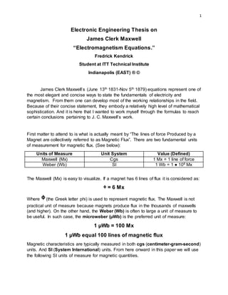
  • 1. 1 Electronic Engineering Thesis on James Clerk Maxwell “Electromagnetism Equations.” Fredrick Kendrick Student at ITT Technical Institute Indianapolis (EAST) ® © James Clerk Maxwell’s (June 13th 1831-Nov 5th 1879) equations represent one of the most elegant and concise ways to state the fundamentals of electricity and magnetism. From them one can develop most of the working relationships in the field. Because of their concise statement, they embody a relatively high level of mathematical sophistication. And it is here that I wanted to work myself through the formulas to reach certain conclusions pertaining to J. C. Maxwell’s work. First matter to attend to is what is actually meant by “The lines of force Produced by a Magnet are collectively referred to as Magnetic Flux”. There are two fundamental units of measurement for magnetic flux. (See below): Units of Measure Unit System Value (Defined) Maxwell (Mx) Cgs 1 Mx = 1 line of force Weber (Wb) SI 1 Wb = 1 ● 108 Mx The Maxwell (Mx) is easy to visualize. If a magnet has 6 lines of flux it is considered as: ᶲ = 6 Mx Where ᶲ(the Greek letter phi) is used to represent magnetic flux. The Maxwell is not practical unit of measure because magnets produce flux in the thousands of maxwells (and higher). On the other hand, the Weber (Wb) is often to large a unit of measure to be useful. In such case, the microweber (µWb) is the preferred unit of measure: 1 µWb = 100 Mx 1 µWb equal 100 lines of magnetic flux Magnetic characteristics are typically measured in both cgs (centimeter-gram-second) units. And SI (System International) units. From here onward in this paper we will use the following SI units of measure for magnetic quantities.
  • 2. 2 Where ▼● is the divergence, ▼x is the curl, π is the constant pi (3.141592654), E is the electric field, B is the magnetic field, p is the charge density, c is the speed of light (299792458 m / s), and J is the vector current density. Modern For time-varying fields, the differential form of these equations in cgs is: Gauss Law for Electricity Gauss Law for Magnetism Faradays Law Maxwell Ampere Law 137 Years Old Table
  • 3. 3 Gauss’ Law for Electricity: The electric flux out of any closed surface is proportional to the total charge enclosed within the surface. Gauss’ Law for Magnetism: The net magnetic flux out of any closed surface is zero. Faraday’s Law of Induction: The line integral of the electric field around a closed loop (the voltage) is equal to the negative of the rate of change of the magnetic flux through the area enclosed by the loop. Ampere’s Law: In the case of static electric field, the line integral of the magnetic field around a closed loop is proportional to the electric current flowing through the loop. Example
  • 4. 4 The displacement current. At a certain instant, a parallel plate capacitor, rated at 17.4 µF, has a potential of 50.0 V across its plates. The area of the plate is 5.00●10.2 m2. If it takes a time of 0.500 s to reach this 50.0-V potential, find (a) the charge deposited on the plates of the capacitor, (b) the average conduction current at that time, (c) the average displacement current at that time, and (d) the rate at which the electric field between the plates is changing at that time. Solution The charge deposited on the plates is: q = CV q = (17.4●106 F) (50.0V) q = 8.70●104 C q = (17.4 • 106 F) (50. V) q = 8.7×10⁴ C q == (1.74 F) • (50. V) q == 87000. C {q = 0.||F V = 1.14943 • 10-9 , C = 0.0000114943 q, C = 10000.F q V} {q == 0. || F V == 1.1494252873563218,C == 0.0000114943 q, C == 10000. F q V} {q = 8.7 • 108 F q V+0. I, 87000.C+0. I = q, 87000. C+0. I = 8.7 • 108 F q V+0. I} Complex Expand [{q == 8.7 F q V, 87000. C == q, 87000. C == 8.7 F q V}] {q == (0. + 0. I) + 8.7 F q V, (0. + 0. I) + 87000. C == q, (0. + 0. I) + 87000. C == (0. + 0. I) + 8.7 F q V} q = 87000 C, F = 0, V = 1 / (870000000 F) Reduce [{q == 8.7 F q V, 87000.C == q, 87000.C == 8.7 F q V}, {C, F, q, V}] {q == 87000 C, F = 0, V == 1/ (870000000 F)} Solution for the variable V: V~~ (1.14943 • 10-9 ) / F Solve [q == 8.7 F q V, V] {V == 1.1494252873563218 / F}
  • 5. 5 The current in the circuit, corresponding to that amount of charge flowing in 0.500 s, found from the definition of the conduction current is: Ic = dq/dt Ic = 8.70●10-4 C / 0.500 s Ic = 1.74●103 A 10-(4 °C (degrees Celsius)) / (0.5 seconds) (10^4 °C (degrees Celsius)) / (0.5 seconds) Quantity [10000, "Degrees Celsius"] / Quantity [0.5, "Seconds"] 20000 K/s (kelvins per second) The displacement current across the capacitor is equal to the conduction current entering the capacitor, therefore: ID = Ic = 1.74●103 A The rate at which the electric field between the plates is changing with time is given by rearranging equation: dE/dt = ID / Ɛ0 A dE/dt = 1.74●10-3 A / (8.85●10-12 C2 / N m2 ) (5.00●10-2 m2 ) (C/s/A) dE = 3.93●109 N/C/s Just as there is a magnetic field around a long straight wire carrying a conduction current, there is a magnetic field around the capacitor associated with a displacement current. Ampère’s law states: Along any arbitrary path encircling a total current Itotal, the integral of the scalar product of the magnetic field B with the element of length dl of the path, is equal to the permeability µ0 times the total current Itotal enclosed by the path. Maxwell reinterpreted Ampère’s law to mean that the total current must be the sum of the
  • 6. 6 conduction current and the displacement current. Thus, Maxwell rewrote Ampère’s law as: ƒB●dI = µo (Ic + ID) With even deeper insight, Maxwell felt that the magnetic field that he associated with the displacement current is more likely associated with the changing electric field with time. In Faraday’s law, it was shown that a changing magnetic field induces an electric field, it is therefore reasonable to assume that the inverse situation also occurs in nature; that is, that a changing electric field can produce a magnetic field. Thus, Maxwell rewrote Ampère’s law in the form of equation (1). But then he added his result for the displacement current found in equation (2). With these modifications, Ampère’s law becomes: (1). ƒB●dI = µo (Ic + ID) (2). ID = ƐO AdE/dt Modified ƒB●dI = µoƐo AdE/dt Ampère’s law says that a magnetic field can be produced by conduction current or a changing electric field with time. As a still further generalization of Ampère’s law, notice that the term AdE/dt in above equation is equal to the change in the electric flux with time. That is, since then: ᶲE = EA dᶲE / dt = AdE/dt Hence, Ampère’s law can be written in the general form: ƒB●dI = µoIc + µoƐo dᶲE/dt As an example of Ampère’s law, let’s determine the magnetic field that exists around a parallel plate capacitor that is caused by the changing electric field within the space between the parallel plates. The parallel plates are circular and have a radius R. Let us
  • 7. 7 determine the magnetic field B at a distance r from the center of the capacitor. Within the capacitor there is no conduction current (i.e., IC = 0). Therefore, Ampère’s law becomes: ƒB●dl = µoƐo A dE/dt Because the magnetic field around a long straight wire carrying a current I is circular, from the point of view of symmetry, it is reasonable to expect that the magnetic field around a displacement current should also be circular, a result that can be proven by experiment. Thus, the magnetic field B is parallel to Δl along the entire circular path. Hence: ƒB●dI = ƒBdI c os 00 = ƒBdl = BƒdI But the sum of the path elements ƒdl is the circumference of the circle, namely 2πr. Therefore: ƒB●dI = B (2πr)
  • 8. 8 Substituting this into Ampère’s law, we get: B (2πr) = µoƐo AdE / dt But B is the area of the parallel plates and is πR2 . Thus: B (2πr) = µoƐo πR2 dE / dt The magnetic field around, and at a distance r from, the capacitor is thus: B = µoƐoR2 (dE) / 2r (dt) [ Notation to: (A - B) & (P – Q) ]
  • 9. 9 Notice that just as the magnetic field around a long straight wire varied as 1/r, so also the magnetic field around the capacitor varies as 1/r. Since µ0 and ε0 are constants of free space, R is the constant radius of the capacitor plate, and for a fixed value of r from the center of the capacitor to the point where the magnetic field is to be determined, we can write the magnetic field at that point as: B = (constant) dE/dt That is, the changing electric field dE/dt is capable of producing a magnetic field B. If the changing electric field within the plates of a capacitor can produce a magnetic field, should not every changing electric field produce a magnetic field? The answer is yes. Hence, there is symmetry in nature. Just as a changing magnetic field can produce an electric field (Faraday’s law); a changing electric field can produce a magnetic field (Ampère’s law as modified by Maxwell). Example A changing electric field with time creates a magnetic field. Find the magnetic field a distance of 20.0 cm from the center of the parallel plate capacitor: Solution The area of the plates of the capacitor (A = πR2) was given as 5.00x10.2 m2, hence the radius of the plate is: R = √A/π R = √5.00●10-2 m2 / π = 0.126 m (1 / 102 m2 (square meters)) / π = 0.126 meters Quantity [0.01, "Meters"] / π == Quantity [0.126, "Meters"] 0.003183 m2 (square meters) = 0.126 meters Quantity [0.003183, "Meters"] == Quantity [0.126, "Meters"]
  • 10. 10 The changing electric field is dE/dt = 3.93 x 10⁹ (N/C)/s. Hence, the magnetic field at a distance of 20.0 cm from the center of the capacitor: E = q/ƐoA B = µoƐoR2 (dE) / 2r (dt) Solution B = µoƐoR2 (dE) / 2r (dt) B = (4π ● 10-7 T m/A) (8.85 ● 10-12 C2 /N m2 ) (0.126 m)2 [3.93 ● 109 (N/C) /s] 2(0.0200 m) B = 1.74x10⁹ T [ Notation: (8.85 x 1027 ) (1.74 x 10⁻³⁴ ) ] Initial Conditions C = 1.74E-05F A = 0.05 m2 Ɛo = 8.85E-12 (C2 ) / N m2 V = 50 V Dt = 0.5 s
  • 11. 11 Solution a). Charge deposited on the plate is 6.15. q = CV q = (1.74E-05F) ● 50V q = 8.70E-04 C b). Current in the circuit, corresponding the amount of charge flowing 0.500 s, found from definition of the conduction current is: Ic = dq / dt Ic = (8.70E-04 C) / (0.5 s) Ic = 1.74E-03 A c). The displacement current is equal to conduction current entering the Capacitor: ID = Ic = 1.74E-03 A d). Rate @ which electric field between the plate is charging, time is given by rearranging equation listed: dE / dt = ID / Ɛo A dE /dt = (1.74E-03 A) / [(8.85E-12(C2 ) / (N m2 ) ● (5.00E-02 m2 )] dE / dt = 3.93E+09 (N/C) / s Derivative: (d) / (dm 2)((1.9661×10⁸ A C2 ) / (N m 2)) = (d(1.9661×10⁸ A C2 ) / (m 2 N)) / (dm 2) Indefinite Integral: ((1.74×10⁻³ A) C2 ) / (8.85×10⁻¹² (N m2 )) dm2 = (1.9661×10⁸ A C2 log (m2 )) / N + constant Changing the electric field with time creates the magnetic field. Distance is 20.0 cm @ the center. Initial Conditions R = 0.20 m
  • 12. 12 Ɛo = 8.85E-12 (C2 ) / N m2 µo = 1.26E-06 (T m) / A Solution (A = πR2 ) = 0.05 m2 is calculated area. The radius is: R = sqrt [A/π] = sprt [(0.05 m2 ) / (3.14159)] = 0.12616 m (0.01592 m2 (square meters) = 0.12616 meters) Charging electric field is dE / dt = 3.93E+09 (N/C) / s. So the field distance now is 20.0 cm: B = [µoƐoR2 dE/dt] [2 r] B = [(1.26E-06 Tm) / A) ● (8.85E-12 (C2 ) / (Nm2 ) (Nm2 ) ● 0.1262 m)2 ● (3.93E+09 N/C) / s)] / [2(0.2 m)] B = 1.74E-09 T Example Magnetic field outside long straight line, what is the distance calculated from 20.0 cm of current? Ic = 1.74 ● 103 A Initial condition: µo = 1.26E-06 (T m) / A I = 1.74E-03 A r = 0.2m
  • 13. 13 Solution: The radius of the magnetic field wire would be 8.48. B = µoIc / 2πr B = (4π ● 10-7 T m / A) (1.74 ● 10-3 A) / 2π (0.200) B = 1.74 ● 10-9 T Alternate form assuming B is real: 1.25664 B+0. I = 1.74 Complex Expand [1.25664 B == 1.74] (0. + 0. I) + 1.25664 B == 1.74 Result: 1.25664 B = 1.74 Source: Michael Faraday (1791-1867) http://skullsinthestars.com/2014/08/27/physics-demonstrations-faraday-disk/ James Clerk Maxwell (1831-1879) http://skullsinthestars.com/2009/07/25/maxwell-on-faraday/ Carl Friedrich Gauss (1777-1855) http://hyperphysics.phy-astr.gsu.edu/hbase/electric/gaulaw.html (The following table summarizes common quantities and their units in both MKS and cgs. Taylor, B. N. "CGS units." §5.3.1 in "Guide for the Use of the International System of Units (SI)." NIST Special Publication 811, p. 11, 1995 Edition. http://physics.nist.gov/Document/sp811.pdf.) http://scienceworld.wolfram.com/physics/cgs.html
  • 14. 14 Jackson, J. D. Classical Electrodynamics, 3rd Ed. New York: Wiley, p. 177, 1998. Z Willinger, D. Handbook of Differential Equations, 3rd ed. Boston, MA: Academic Press, p. 138, 1997. Lorentz Force Law http://hyperphysics.phy-astr.gsu.edu/hbase/magnetic/magfor.html WAV01: Maxwell's Equations – Video https://www.youtube.com/watch?v=Yn-MEMaiA0Y PHYS 101/102 #1: Electromagnetic Waves – Video https://www.youtube.com/watch?v=j2gOh39IyPM “A Student’s Guide to Maxwell’s Equations” DATE PUBLISHED: January 2008 Daniel Fleisch is Associate Professor in the Department of Physics at Wittenberg University, Ohio. His research interests include radar cross-section measurement, radar system analysis, and ground-penetrating radar. He is a member of the American Physical Society (APS), the American Association of Physics Teachers (AAPT), and the Institute of Electrical and Electronics Engineers (IEEE). Cambridge. www.cambridge.org/9780521877619 http://ed.quantum-bg.org/A%20student's%20guide%20to%20maxwell's%20equations- D.%20FleischLEISC.pdf Solution Table Calculation. (Rearranged) Fredrick Kendrick ® © 02/28/2016 Electrical Engineering Student
  • 15. 15 ITT Technical Institute Indianapolis East Campus Don Heller (Electronic Engineer Instructor)