SlideShare a Scribd company logo
1 of 234
Download to read offline
HA − AKU− WSP 1
Wavelets are mathematical functions that cut up data into different frequency compo-
nents, and then study each component with a resolution matched to its scale. They have
advantages over traditional Fourier methods in analyzing physical situations where the
signal contains discontinuities and sharp spikes. Wavelets were developed independently
in the fields of mathematics, quantum physics, electrical engineering, and seismic geology.
Interchanges between these fields during the last years have led to many new wavelet
applications such as image compression, turbulence, human vision, radar, and earthquake
prediction. This course introduces wavelets to the interested technical person outside of
the digital signal processing field. We describe the history of wavelets beginning with
Fourier, compare wavelet transforms with Fourier transforms, state properties and other
special aspects of wavelets, and provide with some interesting applications such as image
compression, interpolation, solution to differential equations, and de-noising noisy data.
The fundamental idea behind wavelets is to analyze according to scale. Indeed, some
researchers in the wavelet field feel that, by using wavelets, one is adopting a whole new
mindset or perspective in processing data.
Wavelets are functions that satisfy certain mathematical requirements and are used in
representing data or other functions. This idea is not new. Approximation using superpo-
sition of functions has existed since the early 1800’s, when Joseph Fourier discovered that
he could superpose sines and cosines to represent other functions. However, in wavelet
analysis, the scale that we use to look at data plays a special role. Wavelet algorithms pro-
cess data at different scales or resolutions. If we look at a signal with a large “window,”
we would notice gross features. Similarly, if we look at a signal with a small “window,”
we would notice small features.
This makes wavelets interesting and useful. For many decades, scientists have wanted
more appropriate functions than the sines and cosines which comprise the bases of Fourier
analysis, to approximate choppy signals. By their definition, these functions are non-local
(and stretch out to infinity). They therefore do a very poor job in approximating sharp
spikes. But with wavelet analysis, we can use approximating functions that are con-
tained neatly in finite domains. Wavelets are well-suited for approximating data with
sharp discontinuities. The wavelet analysis procedure is to adopt a wavelet prototype
function, called an analyzing wavelet or mother wavelet. Temporal analysis is per-
formed with a contracted, high-frequency version of the prototype wavelet,
while frequency analysis is performed with a dilated, low-frequency version of
the same wavelet. Because the original signal or function can be represented in terms of
a wavelet expansion (using coefficients in a linear combination of the wavelet functions),
data operations can be performed using just the corresponding wavelet coefficients. And
if you further choose the best wavelets adapted to your data, or truncate the coefficients
below a threshold, your data is sparsely represented. This sparse coding makes wavelets
an excellent tool in the field of data compression. Other applied fields that are making
use of wavelets include astronomy, acoustics, nuclear engineering, sub-band coding, signal
and image processing, neurophysiology, music, magnetic resonance imaging, speech dis-
crimination, optics, fractals, turbulence, earthquake-prediction, radar, human vision, and
pure mathematics applications such as solving partial differential equations.
HISTORICAL PERSPECTIVE
AKUH· AMIN DAVAR
, Fall-1390, WSP 2
a0 +
∞
X
k=1
(ak cos kx + bk sin kx)
where
a0 =
1
2π
Z 2π
0
f(x)dx, ak =
1
π
Z 2π
0
f(x) cos(kx)dx, ak =
1
2π
Z π
0
f(x) sin(kx)dx,
Fourier’s assertion played an essential role in the evolution of the ideas mathematicians
had about the functions. He opened up the door to a new functional universe.
After 1807, by exploring the meaning of functions, Fourier series convergence, and
orthogonal systems, mathematicians gradually were led from their previous notion of
frequency analysis to the notion of scale analysis. That is, analyzing f(x) by creating
mathematical structures that vary in scale. We construct a function, shift it by some
amount, and change its scale. Apply that structure in approximating a signal. Now
repeat the procedure. Take that basic structure, shift it, and scale it again. Apply it to
the same signal to get a new approximation. And so on. It turns out that this sort of
scale analysis is less sensitive to noise because it measures the average fluctuations of the
signal at different scales.
The first mention of wavelets appeared in an appendix to the thesis of A. Haar (1909).
One property of the Haar wavelet is that it has compact support, which means that it
vanishes outside of a finite interval. Unfortunately, Haar wavelets are not continuously
differentiable which somewhat limits their applications.
In the 1930s, several groups working independently researched the representation of
functions using scale-varying basis functions. Understanding the concepts of basis func-
tions and scale-varying basis functions is key to understanding wavelets; in below provides
a short detour lesson for those interested. By using a scale-varying basis function called
the Haar basis function (more on this later) Paul Levy, a 1930s physicist, investigated
Brownian motion, a type of random signal (2). He found the Haar basis function supe-
rior to the Fourier basis functions for studying small complicated details in the Brownian
motion.
Another 1930s research effort by Littlewood, Paley, and Stein involved computing the
energy of a function f(x):
energy =
1
2
Z 2π
0
|f(x)|2
dx
The computation produced different results if the energy was concentrated around a few
points or distributed over a larger interval. This result disturbed the scientists because it
indicated that energy might not be conserved. The researchers discovered a function that
can vary in scale and can conserve energy when computing the functional energy. Their
work provided David Marr with an effective algorithm for numerical image processing
using wavelets in the early 1980s.
What are Basis Functions?
AKUH· AMIN DAVAR
, Fall-1390, WSP 3
It is simpler to explain a basis function if we move out of the realm of analog (functions)
and into the realm of digital (vectors) (*).
Every two-dimensional vector (x; y) is a combination of the vector (1; 0) and (0; 1): These
two vectors are the basis vectors for (x, y): Why? Notice that x multiplied by (1; 0) is
the vector (x, 0); and y multiplied by (0; 1) is the vector (0; y) : The sum is (x, y) : The
best basis vectors have the valuable extra property that the vectors are perpendicular, or
orthogonal to each other. For the basis (1; 0) and (0; 1); this criteria is satisfied. Now
let’s go back to the analog world, and see how to relate these concepts to basis functions.
By choosing the appropriate combination of sine and cosine function terms whose inner
product add up to zero. The particular set of functions that are orthogonal and that
construct f(x) are our orthogonal basis functions for this problem.
What are Scale-varying Basis Functions?
A basis function varies in scale by chopping up the same function or data space using
different scale sizes. For example, imagine we have a signal over the domain from 0 to 1.
We can divide the signal with two step functions that range from 0 to 1/2 and 1/2 to 1.
Then we can divide the original signal again using four step functions from 0 to 1/4, 1/4
to 1/2, 1/2 to 3/4, and 3/4 to 1. And so on. Each set of representations code the original
signal with a particular resolution or scale.
Between 1960 and 1980, the mathematicians Guido Weiss and Ronald R. Coifman
studied the simplest elements of a function space, called atoms, with the goal of finding
the atoms for a common function and finding the “assembly rules” that allow the recon-
struction of all the elements of the function space using these atoms. In 1980, Grossman
and Morlet, a physicist and an engineer, broadly defined wavelets in the context of quan-
tum physics. These two researchers provided a way of thinking for wavelets based on
physical intuition.
In 1985, Stephane Mallat gave wavelets an additional jump-start through his work
in digital signal processing. He discovered some relationships between quadrature mirror
filters, pyramid algorithms, and orthonormal wavelet bases (more on these later). Inspired
in part by these results, Y. Meyer constructed the first non-trivial wavelets. Unlike the
Haar wavelets, the Meyer wavelets are continuously differentiable; however they do not
have compact support. A couple of years later, Ingrid Daubechies used Mallat’s work to
construct a set of wavelet orthonormal basis functions that are perhaps the most elegant,
and have become the cornerstone of wavelet applications today.
FOURIER ANALYSIS
Fourier’s representation of functions as a superposition of sines and cosines has become
ubiquitous for both the analytic and numerical solution of dierential equations and for
the analysis and treatment of communication signals. Fourier and wavelet analysis have
some very strong links.
FOURIER TRANSFORMS
The Fourier transform’s utility lies in its ability to analyze a signal in the time domain
for its frequency content. The transform works by first translating a function in the time
domain into a function in the frequency domain. The signal can then be analyzed for its
frequency content because the Fourier coefficients of the transformed function represent
the contribution of each sine and cosine function at each frequency. An inverse Fourier
AKUH· AMIN DAVAR
, Fall-1390, WSP 4
transform does just what you’d expect, transform data from the frequency domain into
the time domain.
DISCRETE FOURIER TRANSFORMS
The discrete Fourier transform (DFT) estimates the Fourier transform of a function
from a finite number of its sampled points. The sampled points are supposed to be typical
of what the signal looks like at all other times.
The DFT has symmetry properties almost exactly the same as the continuous Fourier
transform. In addition, the formula for the inverse discrete Fourier transform is easily
calculated using the one for the discrete Fourier transform because the two formulas are
almost identical.
WINDOWED FOURIER TRANSFORMS(WFT)
If f(t) is a nonperiodic signal, the summation of the periodic functions, sine and co-
sine, does not accurately represent the signal. You could artificially extend the signal to
make it periodic but it would require additional continuity at the endpoints. The win-
dowed Fourier transform (WFT) is one solution to the problem of better representing the
nonperiodic signal. The WFT can be used to give information about signals simultane-
ously in the time domain and in the frequency domain. With the WFT, the input signal
f(t) is chopped up into sections, and each section is analyzed for its frequency content
separately. If the signal has sharp transitions, we window the input data so that the
sections converge to zero at the endpoints. This windowing is accomplished via a weight
function that places less emphasis near the interval’s endpoints than in the middle. The
effect of the window is to localize the signal in time. The short-time Fourier transform
(STFT), or alternatively short-term Fourier transform, is a Fourier-related transform used
to determine the sinusoidal frequency and phase content of local sections of a signal as it
changes over time.
STFT {x(t)} ≡ X(τ, ω) =
Z ∞
−∞
x(t)w(t − τ)e−jωt
dt
where w(t) is the window function, commonly a Hann window or Gaussian “hill” centered
around zero, and x(t) is the signal to be transformed. X(τ, ω) is essentially the Fourier
Transform of x(t)w(t − τ), a complex function representing the phase and magnitude of
the signal over time and frequency. Often phase unwrapping is employed along either or
both the time axis, τ, and frequency axis, ω, to suppress any jump discontinuity of the
phase result of the STFT. The time index τ is normally considered to be ”slow” time and
usually not expressed in as high resolution as time t.
Discrete-time STFT
STFT {x[n]} ≡ X(m, ω) =
∞
X
n=−∞
x[n]w[n − m]e−jωn
In this case, m is discrete and ω is continuous, but in most typical applications the STFT
is performed on a computer using the Fast Fourier Transform(FFT), so both variables
are discrete and quantized.
AKUH· AMIN DAVAR
, Fall-1390, WSP 5
The magnitude squared of the STFT yields the spectrogram of the function:
spectrogram {x(t)} ≡ |X(τ, ω)|2
Inverse STFT
Given the width and definition of the window function w(t), we initially require the height
of the window function to be scaled so that
Z ∞
−∞
w(τ) dτ = 1 ⇒
Z ∞
−∞
w(t − τ) dτ = 1 ∀ t
x(t) = x(t)
Z ∞
−∞
w(t − τ) dτ =
Z ∞
−∞
x(t)w(t − τ) dτ.
X(ω) =
Z ∞
−∞
x(t)e−jωt
dt.
X(ω) =
Z ∞
−∞
Z ∞
−∞
x(t)w(t − τ) e−jωt
dt dτ (1)
=
Z ∞
−∞
Z ∞
−∞
x(t)w(t − τ) e−jωt
dt

dτ (2)
=
Z ∞
−∞
X(τ, ω) dτ. (3)
Since the inverse Fourier transform is
x(t) =
1
2π
Z ∞
−∞
X(ω)ejωt
dω =
1
2π
Z ∞
−∞
Z ∞
−∞
X(τ, ω)ejωt
dτ dω.
comparing to above that windowed x(t) or “wavelet” of x(t) is
x(t)w(t − τ) =
1
2π
Z ∞
−∞
X(τ, ω)ejωt
dω.
the inverse Fourier transform of X(τ, ω) for τ fixed.
To numerically evaluate the STFT, we sample the frequency ω in N equally spaced samples
from 0 ≤ ω ≤ 2π, ωk = 2πk/N, 0 ≤ k ≤ N − 1
X(k, m) = X(2πk/N, m) =
R−1
X
n=0
x(n − m)w(n)e−j2πk/Nn
, k = 0, 1, · · · , N − 1
= DFTN



x(n − m)w(n)|R−1
n=0 , 0, 0, · · · , 0
| {z }
N−R



FAST FOURIER TRANSFORMS
To approximate a function by samples, and to approximate the Fourier integral by
the discrete Fourier transform, requires applying a matrix whose order is the number
AKUH· AMIN DAVAR
, Fall-1390, WSP 6
sample points n : Since multiplying an n × n matrix by a vector costs on the order of
n2
arithmetic operations, the problem gets quickly worse as the number of sample points
increases. However, if the samples are uniformly spaced, then the Fourier matrix can be
factored into a product of just a few sparse matrices, and the resulting factors can be
applied to a vector in a total of order n log n arithmetic operations. This is the so-called
Fast Fourier transform or (FFT).
WAVELET TRANSFORMS VERSUS FOURIER TRANSFORMS
SIMILARITIES BETWEEN FOURIER AND WAVELET TRANSFORMS
The fast Fourier transform (FFT) and the discrete wavelet transform (DWT) are both
linear operations that generate a data structure that contains log2 n segments of various
lengths, usually filling and transforming it into a different data vector of length 2n
. The
mathematical properties of the matrices involved in the transforms are similar as well.
The inverse transform matrix for both the FFT and the DWT is the transpose of the
original. As a result, both transforms can be viewed as a rotation in function space to a
different domain. For the FFT, this new domain contains basis functions that are sines
and cosines. For the wavelet transform, this new domain contains more complicated basis
functions called wavelets, mother wavelets, or analyzing wavelets.
Both transforms have another similarity. The basis functions are localized in frequency,
making mathematical tools such as power spectra (how much power is contained in a
frequency interval) and scalegrams (to be defined later) useful at picking out frequencies
and calculating power distributions.
DISSIMILARITIES BETWEEN FOURIER AND WAVELET TRANSFORMS
The most interesting dissimilarity between these two kinds of transforms is that indi-
vidual wavelet functions are localized in space. Fourier sine and cosine functions are not.
This localization feature, along with wavelets’ localization of frequency, makes many func-
tions and operators using wavelets “sparse” when transformed into the wavelet domain.
This sparseness, in turn, results in a number of useful applications such as data compres-
sion, detecting features in images, and removing noise from time series. One way to see
the time-frequency resolution differences between the Fourier transform and the wavelet
transform is to look at the basis function coverage of the time-frequency plane. Figure
7 shows a windowed Fourier transform, where the window is simply a square wave. The
square wave window truncates the sine or cosine function to fit a window of a particular
width. Because a single window is used for all frequencies in the WFT(windowed Fourier
transform, the resolution of the analysis is the same at all locations in the time-frequency
plane.
One of the downfalls of the STFT is that it has a fixed resolution. The width of
the windowing function relates to how the signal is representedit determines
whether there is good frequency resolution (frequency components close to-
gether can be separated) or good time resolution (the time at which frequen-
cies change). A wide window gives better frequency resolution but poor time resolution.
A narrower window gives good time resolution but poor frequency resolution. These are
called narrowband and wideband transforms, respectively.
AKUH· AMIN DAVAR
, Fall-1390, WSP 7
Time
Frequency
Figure 1: Better time resolution
Example
Using the following sample signal x(t) that is composed of a set of four sinusoidal
waveforms joined together in sequence. Each waveform is only composed of one of four
frequencies (10, 25, 50, 100 Hz). The definition of x(t) is:
x(t) =







cos(2π10t),
cos(2π25t),
cos(2π50t),
cos(2π100t),
N=400; t1=linspace(0,1,N);
s1=cos(2*pi*10*t1);s2=cos(2*pi*20*t1);s3=cos(2*pi*40*t1);s4=cos(2*pi*80*t1);
plot(t1,s1,t1+1,s2,t1+2,s3,t1+3,s4)
plot(linspace(-200,200,4*400),abs(fftshift(fft([s1 s2 s3 s4])))); grid; figure(gcf)
Let’s determine the spectral behavior using FFT
plot(linspace(-200,200,4*400),abs(fftshift(fft([s1 s2 s3 s4])))); grid; figure(gcf)
From figure 3, as we observe, there is no information as to the spectral behavior of
sinusoidal signals(how many? what frequencies?). On the other hand, from figure 4, there
is no information as to the beginning and end of each sinusoids though the frequencies
are determined. In figure 6 we observe that each signal there is only one specific
frequency centered around (10,20,40,80) for all times.
AKUH· AMIN DAVAR
, Fall-1390, WSP 8
Time
Frequency
Figure 2: Better frequency resolution
subplot(221); spectrogram([s1],’’,0,256,400);title(’a’); figure(gcf)
subplot(222); spectrogram([s2],’’,0,256,400);title(’b’); figure(gcf)
subplot(223); spectrogram([s3],’’,0,256,400);title(’c’); figure(gcf)
subplot(224); spectrogram([s4],’’,0,256,400);title(’d’); figure(gcf)
Concatenation of the four sinusoids in time and frequency are distinguished using
spectrogram([s1 s2 s3 s4],’’,0,256,400); figure(gcf)
In mathematics, a wavelet series is a representation of a square-integrable (real- or
complex-valued) function by a certain orthonormal series generated by a wavelet.
A function ψ ∈ L2
(R) is called an orthonormal wavelet if it can be used to define
a Hilbert basis, that is a complete orthonormal system, for the Hilbert space L2
(R) of
square integrable functions. The Hilbert basis is constructed as the family of functions
{ψjk : j, k ∈ Z} by means of dyadic translations and dilations of ψ,
ψjk(x) = 2j/2
ψ(2j
x − k)
for integers j, k ∈ Z. This family is an orthonormal system if it is orthonormal under
the inner product
hψjk, ψlmi = δjlδkm
where δjl is the Kronecker delta and hf, gi is the standard inner product hf, gi =
R ∞
−∞
f(x)g(x)dx
on L2
(R). The requirement of completeness is that every function f ∈ L2
(R) may be ex-
panded in the basis as
f(x) =
∞
X
j,k=−∞
cjkψjk(x)
AKUH· AMIN DAVAR
, Fall-1390, WSP 9
0 0.5 1 1.5 2 2.5 3 3.5 4
−1
−0.8
−0.6
−0.4
−0.2
0
0.2
0.4
0.6
0.8
1
Time, sec.
Figure 3: Concatenation of some sinusoids in time domain.
−200 −150 −100 −50 0 50 100 150 200
0
50
100
150
200
250
freq., Hz
Figure 4: Spectral behavior of concatenation of the sinusoids in frequency domain.
AKUH· AMIN DAVAR
, Fall-1390, WSP 10
0 50 100 150 200
0.2
0.4
0.6
0.8
Frequency (Hz)
a
Time
0 50 100 150 200
0.2
0.4
0.6
0.8
Frequency (Hz)
b
Time
0 50 100 150 200
0.2
0.4
0.6
0.8
Frequency (Hz)
c
Time
0 50 100 150 200
0.2
0.4
0.6
0.8
Frequency (Hz)
d
Time
Figure 5: Time-frequency analysis of each individual sinusoids.
0 50 100 150 200
0.5
1
1.5
2
2.5
3
3.5
Frequency (Hz)
Time
Figure 6: Time-frequency analysis four concatenated sinusoids.
AKUH· AMIN DAVAR
, Fall-1390, WSP 11
Time
Frequency
Figure 7: Fourier basis functions, time-frequency tiles, and coverage of the time-frequency
plane
with convergence of the series understood to be convergence in norm. Such a repre-
sentation of a function f is known as a wavelet series. This implies that an orthonormal
wavelet is self-dual. The integral wavelet transform is the integral transform defined as
[Wψf] (a, b) =
1
p
|a|
Z ∞
−∞
ψ

x − b
a

f(x)dx
The wavelet coefficients cjk are then given by
cjk = [Wψf] (2j
, k2j
)
Here, a = 2j
is called the binary dilation or dyadic dilation, and b = k2j
is the binary
or dyadic position.
Introduction to the world of transform
A mathematical operation that takes a function or sequence and maps into another one
f(x) =
Z
F(w)K(w, x)dw
AKUH· AMIN DAVAR
, Fall-1390, WSP 12
fj =
X
j
KijFi
Examples:
Laplace, Fourier, DTFT, DFT, FFT, z-transform Fourier Transform
X(f) =
Z ∞
−∞
x(t)e−2jπft
dt
x(t) =
Z ∞
−∞
X(f)e2jπft
df
Fourier transform identifies all spectral components present in the signal, however it
does not provide any information regarding the temporal (time) localization of the
components.
Fourier Transform : Limitations
1. Signals are of two types
(a) Stationary
(b) Non-stationary
2. Non-stationary signals are those who have got time varying spectral components
. . . FT gives only provides the existence of the spectral components of the signal
. . . But does not provide any information on the time occurrence of spectral compo-
nents
3. The basis function e−jωt
stretches to infinity, Hence, only analyzes the signal globally.
4. In order to obtain time-localization of spectral components, the signal need to be
analyzed locally.
Time–Frequency Representation
1. Instantaneous frequency:
fx(t) =
1
2π
d
dt
∠x(t)
2. Group delay:
tx(f) = −
1
2π
d
df
∠X(f)
3. Disadvantages of above expressions: These equations though have a huge theoretical
significance but are not easy to implement.
4. All time-frequency-energy representations should be classified as time-frequency
analysis; thus, wavelet, Wigner-Ville Distribution and spectrogram should all be
included.
AKUH· AMIN DAVAR
, Fall-1390, WSP 13
5. Almost by default, the term, time-frequency analysis, was monopolized by the
Wigner-Ville distribution.
6. To have a valid time-frequency representation, we have to have frequency and energy
functions varying with time. Therefore, the frequency and energy functions should
have instantaneous values
Wigner-Ville Distribution
Wigner-Ville Distribution, W(ω, t), is defined as
W(ω, t) =
1
2π
Z ∞
−∞
x(t − τ/2)x(t + τ/2) e−jωτ
dτ
E{W(ω, t)} =
1
2π
Z ∞
−∞
E{x(t)x(t + τ)} e−jωτ
dτ
=
1
2π
Z ∞
−∞
Rxx(t, τ) e−jωτ
dτ
WV Instantaneous Frequency
ω(t) =
R ∞
−∞
ωW(ω, t) dω
R ∞
−∞
W(ω, t) dω
7. Therefore, at any given time, there is only one instantaneous frequency value.
8. What if there are two independent components? In this case, VW gives the weighted
mean.
If x(t) = x1(t) + x2 (t) then
S(ω) = S1(ω) + S2(ω) ,
where S(ω) = 1
√
2π
R
t
x(t) e−iωt
d t .
|S|2
= |S1 + S2|2
= |S1|2
+ |S2|2
+ 2ℜ [S∗
1S2]
6= |S1|2
+ |S2|2
.
Short-time Fourier Transform
STFTw
x (τ, w) =
Z
t
[x(t)w(t − τ)]e−jwt
dt
AKUH· AMIN DAVAR
, Fall-1390, WSP 14
• w(t) : windowing function generally a Gaussian pulse is used, other choices are
rectangular, elliptic etc . . .
• Maps 1D function to 2D time-frequency domain
• Advantages:
– Gives us time-frequency description of the signal
– Overcomes the difficulties of Fourier transform by use of windowing functions
STFT: Disadvantages
• Heisenberg Principle: One can not get infinite time and frequency resolution beyond
Heisenberg’s Limit
∆t ∆f ≥
1
4π
, ♣
where
∆t =
sR ∞
−∞
t2|g(t)|2dt
R ∞
−∞
|g(t)|2dt
, ∆f =
sR ∞
−∞
f2|G(f)|2df
R ∞
−∞
|G(f)|2df
Proof using Schwartz inequality:
Z ∞
−∞
g1(s)g2(s)ds
2
≤
Z ∞
−∞
g2
1(u)du
Z ∞
−∞
g2
2(u)du
Let’s g1(t) = tg(t), g2(t) = g′
(t) ⇒
Z ∞
−∞
tg(t)g′
(t)dt
2
≤
Z ∞
−∞
t2
g2
(t)dt
Z ∞
−∞
[g′
(t)]2
dt
[g′
(t)]2 F
←→[j2πfG(f)] ∗ [j2πfG(f)] = −4π2
Z ∞
−∞
νG(ν)(f − ν)G(f − ν)dν ⇒
Z ∞
−∞
[g′
(t)]2
dt = 4π2
Z ∞
−∞
ν2
|G(ν)|2
dν
g2
(t)
F
←→ G(f) ∗ G(f)
2g′
(t)g(t)
F
←→ j2πf[G(f) ∗ G(f)]
Z ∞
−∞
g(t)g′
(t)e−j2πft
dt = jπf
Z ∞
−∞
G(ν)G(f − ν)dν ⇒
Z ∞
−∞
(−j2πt)g(t)g′
(t) e−j2πft
f=0
dt = jπ
Z ∞
−∞
G(ν)G(f − ν)
f=0
dν+

jπf
Z ∞
−∞
G(ν)G′
(f − ν)dν
f=0
−2
Z ∞
−∞
tg(t)g′
(t)dt =
Z ∞
−∞
G(ν)G(−ν)dν =
Z ∞
−∞
|G(f)|2
df
AKUH· AMIN DAVAR
, Fall-1390, WSP 15
−2
Z ∞
−∞
tg(t)g′
(t)dt =
Z ∞
−∞
|G(f)|2
df
Z ∞
−∞
tg(t)g′
(t)dt
2
≤
Z ∞
−∞
t2
g2
(t)dt
Z ∞
−∞
4π2
f2
|G(f)|2
df
Divide both sides by E2
g =
Z ∞
−∞
g2
(t)dt
2
=
Z ∞
−∞
|G(f)|2
df
2
to have the desired
result ♣. The function that satisfies ♣ with equality is Gaussian:
g1(t) = K0g2(t) ⇒ tg(t) = K0g′
(t) ⇒ g(t) = K1et2/K0
• Trade offs:
– Wider window: Good frequency resolution, Poor time resolution
– Narrower window: Good time resolution, Poor frequency resolution
The definition of the class of bilinear (or quadratic) time-frequency distributions:
Cx(t, f) =
Z ∞
−∞
Z ∞
−∞
Ax(η, τ)Φ(η, τ) exp(−j2π(ηt + τf)) dη dτ,
where Ax (η, τ) is the ambiguity function .
Φ (η, τ) is the kernel function which is usually a low-pass function and is used to mask
out the interference.
The class of bilinear (or quadratic) time-frequency distributions can be most easily
understood in terms of the ambiguity function an explanation of which follows.
Consider the well known power spectral density Px (f) and the signal auto-correlation
function Rx (τ) in the case of a stationary process. The relationship between these
Px(f) =
Z ∞
−∞
Rx(τ)ej2πfτ
dτ, (4)
Rx(τ) = E{x(t + τ/2)x∗
(t − τ/2)} (5)
For a non-stationary signal x (t) , these relations can be generalized using a
time-dependent power spectral density or equivalently the famous Wigner
distribution function of x (t) as follows:
Wx(t, f) =
Z ∞
−∞
Rx(t, τ)e−j2πfτ
dτ, (6)
Rx (t, τ) = E{x(t + τ/2)x(t − τ/2)}. (7)
If the Fourier transform of the auto-correlation function is taken with respect to t
instead of τ, we get the ambiguity function as follows:
Ax(η, τ) =
Z ∞
−∞
x(t + τ/2)x∗
(t − τ/2)ej2πtη
dt.
AKUH· AMIN DAVAR
, Fall-1390, WSP 16
Ax(η, τ)
FtF−1
f
Fτ F−1
η
Wx(t, f)
Rx(t, τ)
Ft
F−1
η
F−1
f
Fτ
Figure 8: The relationship between the Wigner distribution function, the auto-
correlation function and the ambiguity function.
Linear vs. Quadratic Distributions
Linear: Quadratic
Pros: Pros:
Linear superposition Better time and frequency resolutions than linear
No interference terms for muti-component signals Shows the energy distribution
Cons: Cons:
Trade off between time and frequency resolutions Cross terms for multi-component signals
Heisenberg inequality
Wavelet Transform
• Overcomes the shortcoming of STFT by using variable length windows: i.e. Nar-
rower window for high frequency thereby giving better time resolution and Wider
window at low frequency thereby giving better frequency resolution
• Heisenberg’s Principle still holds
• Mathematical formula:
CWTΨ
x (τ, s) = Ψ(τ, s) =
1
p
|s|
Z
t
x(t)Ψ∗
(
t − τ
s
)dt
where
AKUH· AMIN DAVAR
, Fall-1390, WSP 17
Absolute Values of Ca,b Coefficients for a = 0.01 1.02 2.03 3.04 4.05 ...
time (or space) b
scales
a
100 200 300 400 500 600
0.01
5.06
10.11
15.16
20.21
25.26
30.31
35.36
40.41
45.46
50.51
55.56
60.61
65.66
70.71
75.76
80.81
85.86
90.91
95.96
50
100
150
200
Figure 9: Continuous wavelet of δ(t) for small scales(large frequencies) around 400 are
strong and as we move away from b = 400 there is conic relationship between scales and
delays.
x(t) = given signal
τ = translation parameter
s = scaling parameter = 1/f
Ψ(t) = Mother wavelet , All kernels are obtained by scaling
and/or translating mother wavelet
Example using Morlet wavelet Ψ(t) = cos(5t)e−t2/2
:
x=[zeros(1,400) 1 zeros(1,199)];
s=cwt(x,linspace(1e-2,100,100),’morl’,’plot’);
figure(gcf);pause;
colormap(’default’);
X=linspace(0,100,100);Y=0:599;
contour(Y,X,s);figure(gcf);pause;
mesh(Y,X,s);figure(gcf)
x=cos(2*pi*5*(0:199)/200);
s=cwt(x,linspace(1e-2,50,100),’morl’,’plot’);
figure(gcf);pause;colormap(’default’);
X=linspace(1e-2,50,100);Y=0:199;contour(Y,X,s);
figure(gcf);pause; mesh(Y,X,s);figure(gcf)
AKUH· AMIN DAVAR
, Fall-1390, WSP 18
0 100 200 300 400 500
0
10
20
30
40
50
60
70
80
90
100
−0.4
−0.3
−0.2
−0.1
0
0.1
0.2
0.3
0.4
Figure 10: Contour plot of wavelet of δ(t), for scales less than 30 wavelet vales of δ(t) are
large around b = 400.
Figure 11: Mesh plot of wavelet of δ(t).
AKUH· AMIN DAVAR
, Fall-1390, WSP 19
Absolute Values of Ca,b Coefficients for a = 0.01 0.51495 1.0199 1.5248 2.0298 ...
time (or space) b
scales
a
50 100 150 200
0.01
2.53475
5.05949
7.58424
10.109
12.6337
15.1585
17.6832
20.208
22.7327
25.2575
27.7822
30.307
32.8317
35.3565
37.8812
40.406
42.9307
45.4555
47.9802
50
100
150
200
Figure 12: Continuous wavelet of cos(2π5t) for small scales around 30 for almost all delays
is strong but we observe some repetition in x−axis.
0 50 100 150
5
10
15
20
25
30
35
40
45
50
−6
−4
−2
0
2
4
6
Figure 13: Contour plot of wavelet of cos(2π5t), for scales around 30 wavelet vales of δ(t)
are strong.
AKUH· AMIN DAVAR
, Fall-1390, WSP 20
0
50
100
150
200
0
20
40
60
−10
−5
0
5
10
−6
−4
−2
0
2
4
6
Figure 14: Mesh plot of wavelet of cos(2π5t).
close all
t=linspace(0,1,100); x=[sin(2*pi*5*t)];
figure(1)
cw1 = cwt(x,1:30,’morl’,’plot’);
title(’Continuous Transform, absolute coefficients.’)
ylabel(’Scale’)
figure(2)
%[cw1,sc] = cwt(x,1:40,’morl’,’scal’);
[cw1,sc] = cwt(x,1:30,’morl’,’scalCNT’);
title(’Scalogram’)
ylabel(’Scale’)
figure(gcf)
close all
t=linspace(0,1,100); x=[sin(2*pi*5*t) sin(2*pi*15*t) sin(2*pi*25*t)];
figure(1)
cw1 = cwt(x,1:30,’morl’,’plot’);
title(’Continuous Transform, absolute coefficients.’)
ylabel(’Scale’)
figure(2)
%[cw1,sc] = cwt(x,1:40,’morl’,’scal’);
[cw1,sc] = cwt(x,1:30,’morl’,’scalCNT’);
title(’Scalogram’)
AKUH· AMIN DAVAR
, Fall-1390, WSP 21
ylabel(’Scale’)
figure(gcf)
Scale values determine the degree to which the wavelet is compressed or stretched. Low
scale values compress the wavelet and correlate better with high frequencies. The low
scale CWT coefficients represent the fine-scale features in the input signal vector. High
scale values stretch the wavelet and correlate better with the low frequency content of
the signal. The high scale CWT coefficients represent the coarse-scale features in the
input signal.
Continuous Wavelet transform
• The kernel functions used in wavelet transform are all obtained from one prototype
function known as mother wavelet, by scaling and/or translating it.
Ψa,b(t) =
1
√
a
Ψ(
t − b
a
)
a = scale parameter
b = translation parameter
Ψ1,0(t) = Ψ(t)
• Continuous Wavelet transform
W(a, b) =
1
√
a
Z ∞
−∞
x(t)Ψa,b(t)dt
• In order to become a wavelet a function must satisfy the above two conditions
Z ∞
−∞
Ψ(t)dt = 0
Z ∞
−∞
|Ψ(t)|2
dt  ∞
Inverse wavelet transform
x(t) =
1
C
Z ∞
−∞
Z ∞
−∞
1
a2
W(a, b)Ψa,b(t)dadb
where
C =
Z ∞
−∞
|Ψ(w)|
|w|
dw
provided
Z ∞
−∞
Ψ(t)dt = 0
AKUH· AMIN DAVAR
, Fall-1390, WSP 22
Proof:
f(ω) =
1
2π
Z ∞
−∞
f(t)e−jωt
dt, Fourier transform
F(ω, s) =
1
2π
Z ∞
−∞
f(t)g(t − s)e−jωt
dt, Windowed transform
For each s, we recover f(t)g(t − s) by
f(t)g(t − s) =
Z ∞
−∞
F(ω, s)ejωt
dω
Multiply both sides by g∗
(t − s) and integrate over s.
f(t)
Z ∞
−∞
g(t − s)g∗
(t − s)ds =
Z ∞
−∞
Z ∞
−∞
F(ω, s)g∗
(t − s)ejωt
dωds
f(t) =
1
||g(t)||2
Z ∞
−∞
Z ∞
−∞
F(ω, s)g∗
(t − s)ejωt
dωds
This is the reconstruction from time-frequency(space) transform.
So far we concentrated on windowed STFT.
Wavelets begin with one function Ψ(t). The position variable s still comes from
translation Ψ(t − s). Now comes the difference. Instead of the frequency variable we have
a scale variable.
Instead of modulating them we rescale them. The “time-scale atoms” are the translates
and dilates of Ψ(t) :
Ψa,b(t) =
1
√
a
Ψ((t − b)/a), Wavelet functions
The mother wavelet is Ψ(t) = Ψ1,0(t). The factor |a|−0.5
assures that rescaled wavelets
have equal energy ||Ψa,b(t)|| = ||Ψ(t)||. We normalize so that all these functions have
unit norm ||Ψa,b(t)|| = 1.
Scaling the time by aj
automatically scales the translation steps by a−j
Ψ(aj
t − k) = Ψ(aj
[t − a−j
k])
The mesh length at level j is scaled down by a−j
. The frequency is scaled up by aj
. This
hyperbolic scaling or dyadic scaling or octave scaling (a = 2) is a prime characteristic of
wavelet analysis.
Any smooth decaying function Ψ(t) is a mother wavelet provided that
Z
Ψ(t)dt = 0
F
n
Wf (a, b) = f(t) ∗
p
|a|−1Ψ(−t/a)
o
=
p
|a|F(ω)Ψ∗
(aω)
AKUH· AMIN DAVAR
, Fall-1390, WSP 23
F
nh
Wg(a, b) = g(t) ∗
p
|a|−1Ψ(−t/a)
i∗o
=
p
|a|G∗
(ω)Ψ(aω)
Wf (a, b) ←→
p
|a|F(ω)Ψ∗
(aω)
W∗
g (a, b) ←→
p
|a|G(ω)Ψ(aω)
Multiply Wf (a, b) and W∗
g (a, b) and integrate over b
Z ∞
−∞
Wf (a, b)W∗
g (a, b)db = 2π
Z ∞
−∞
|a|F(ω)G∗
(ω)|Ψ(aω)|2
dω
Integrate this equation with respect to da/|a|2
and reverse the order of integration:
Z ∞
−∞
Z ∞
−∞
Wf (a, b)W∗
g (a, b)
dadb
|a|2
= 2π
Z ∞
−∞
Z ∞
−∞
|a|F(ω)G∗
(ω)|Ψ(aω)|2 dωda
|a|2
, U
2π
Z ∞
−∞
Z ∞
−∞
F(ω)G∗
(ω)|Ψ(aω)|2 dωda
|a|
= 2π
Z ∞
−∞
F(ω)G∗
(ω)dω
Z ∞
−∞
|Ψ(aω)|2 da
|a|
2π
Z ∞
−∞
|Ψ(aω)|2 da
|a|
= 2π
Z ∞
−∞
|Ψ(ω)|2
|ω|
dω
Obtained by ν = aω, dν = ωda, da/|a| = dω/|ω|
Therefore,
Z ∞
−∞
Z ∞
−∞
Wf (a, b)W∗
g (a, b)
dadb
|a|2
= C
Z ∞
−∞
f(t)g∗
(t)dt, C = 2π
Z ∞
−∞
|Ψ(ω)|2
|ω|
dω
By assuming g(t − τ) = δ(t) ⇒ Wg(a, b) = Ψ((τ − b)/a)/
√
a, from equation U we have
Z ∞
−∞
Z ∞
−∞
Wf (a, b)Ψ((τ − b)/a)/
√
a
dadb
|a|2
= C
Z ∞
−∞
f(t)δ(t − τ)dt = Cf(τ) ⇒
f(t) =
1
C
Z ∞
−∞
Z ∞
−∞
Wf (a, b)Ψ((t − b)/a)/
√
a
dadb
|a|2
Example of Meyer wavelet and its Fourier transform
Meyer wavelet is defined in frequency domain, by refering to MATLAB for their
representation:
ψ(ω) =
(
ejω/2
√
2π
sin(0.5v(3|ω|/2π − 1)) 2π
3
≤ |ω| ≤ 4π
3
ejω/2
√
2π
sin(0.5v(3|ω|/4π − 1)) 4π
3
≤ |ω| ≤ 8π
3
ψ(ω) = 0, ω ∋

2π
3
,
8π
3

v(a) = a4
(35 − 84a + 70a2
− 20a3
), a ∈ [0, 1]
φ(x) =
1
√
2π
|ω| ≤
2π
3
φ(x) =
1
√
2π
cos(0.5v(3|ω|/2/π − 1))
2π
3
≤ |ω| ≤
4π
3
φ(x) = 0 |ω| ≥
4π
3
AKUH· AMIN DAVAR
, Fall-1390, WSP 24
−8 −6 −4 −2 0 2 4 6 8
−1
−0.5
0
0.5
1
1.5
Meyer wavelet: ψ(x)
x
ψ(x)
−600 −400 −200 0 200 400 600
−200
−150
−100
−50
0
50
f
F{ψ(x)}
Figure 15: Wavelet ψ and its Fourier transform, they are very much concentrated in time
and frequency domain.
[phi,psi,x] = wavefun(’meyr’,10);
figure(1)
subplot(211)
plot(x,psi);grid;figure(gcf);
title(’Meyer wavelet: $psi(x)$’)
xlabel(’$x$’);ylabel(’$psi(x)$’);
subplot(212)
f=linspace(-.5,.5,length(x))*length(x);
PSI=abs(fftshift(fft(psi)));
plot(f,10*log10(PSI));grid;figure(gcf);
xlabel(’$f$’);ylabel(’$mathcal{F}{psi(x)}$’);
figure(2)
subplot(211)
plot(x,phi);grid;figure(gcf);
title(’Meyer wavelet: $phi(x)$’)
xlabel(’$x$’);ylabel(’$phi(x)$’);
subplot(212)
f=linspace(-.5,.5,length(x))*length(x);
PHI=abs(fftshift(fft(phi)));
plot(f,10*log10(PHI));grid;figure(gcf);
xlabel(’$f$’);ylabel(’$mathcal{F}{phi(x)}$’);
AKUH· AMIN DAVAR
, Fall-1390, WSP 25
−8 −6 −4 −2 0 2 4 6 8
−0.5
0
0.5
1
1.5
Meyerwavelet: φ(x)
x
φ(x)
−600 −400 −200 0 200 400 600
−200
−100
0
100
f
F
{φ(x)}
Figure 16: Scaling function(father wavelet) φ and its Fourier transform, they are very
much concentrated in time and frequency domain.
Constant Q-filtering
• CWT can be rewritten as
W(a, b) = x(b) ∗ Ψ∗
a,0(−b)
Proof:
Ψa,0(t) =
1
√
a
Ψ(t/a) ⇒ Ψa,0(−b) =
1
√
a
Ψ(−b/a)
x(b) ∗ Ψa,0(−b) =
Z ∞
−∞
x(t)
1
√
a
Ψ(−(b − t)/a) = CWTΨ
x (a, b)
• A special property of the above filter defined by the mother wavelet is that they are
Constant-Q filters
• Q factor = Center frequency/Bandwidth
Q = 2π
Energy Stored
Energy dissipated per cycle
= 2πfr
Energy Stored
Power Loss
, fr = resonant frequency
• Hence the filter defined by wavelet increases their Bandwidth as scale increases (
i.e. center frequency increases )
• This leads to filter bank implementation of discrete wavelet transform
AKUH· AMIN DAVAR
, Fall-1390, WSP 26
I. Daubechies believes that the wavelet transform can be used to analyze time series
that contain nonstationary power at many different frequencies.
The term “wavelet function” is used generically to refer to either orthogonal or
nonorthogonal wavelets. The term “wavelet basis” refers only to an
orthogonal set of functions. The use of an orthogonal basis implies the use of the
discrete wavelet transform, while a nonorthogonal wavelet function can be used with
either the discrete or the continuous wavelet transform.
The continuous wavelet transform of a discrete sequence xn is defined as the convolution
of xn with a scaled and translated version of ψ0(t):
Wn(s) =
N−1
X
n′=0
xn′ ψ∗
((n′
− n)δt/s) (8)
in this formula ψ(·) is normalized:
Z ∞
−∞
|ψ̂(ω′
)|2
dω′
= 1
Use of DFT allows to do convolution (8) easily
x̂k =
1
N
N−1
X
n=0
xne−j2πkn/N
Using F{ψ(t/s)} = ψ̂(sω), By the convolution theorem, the wavelet transform is the
inverse Fourier transform of the product:
Wn(s) =
N−1
X
k=0
x̂kψ̂∗
(sωk)ejωknδt
(9)
angular frequency ωk :
ωk =







2πk
Nδt
, k ≤ N
−
2πk
Nδt
, k  N
Using (9), the continuous wavelet transform (for a given s) at all n is calculated
simultaneously and efficiently.
To ensure that the wavelet transforms (9) at each scale s are directly comparable to
each other and to the transforms of other time series, the wavelet function at each scale
s is normalized to have unit energy:
ψ̂(sωk) =
r
2πs
δt
ψ̂0(sωk), ψ((n′
− n)δt/s) =
r
δt
s
ψ((n′
− n)δt/s) (10)
AKUH· AMIN DAVAR
, Fall-1390, WSP 27
Name ψ0(t) ψ̂0(sω)
Morlet
(ω0=frequency)
π−1/4
ejω0t
e−t2/2
π−1/4
H(ω)e−(sω−ω0)2/2
Paul
(m=order)
2mjmm!
√
π(2m)!
(1 − jt)−(m+1) 2m
√
m(2m−1)!
H(ω)(sω)m
e−sω
DOG
(m=derivative)
(−1)m+1
√
Γ(m+1/2)
dm
dtm e−t2/2 −jm
√
Γ(m+1/2)
(sω)m
e−(sω)2/2
Table 1: H(ω) = Heaviside step function, H(ω) = 1 if ω  0, H(ω) = 0 otherwise. DOG
= derivative of a Gaussian; m = 2 is the Marr or Mexican hat wavelet.
Some of the unscaled ψ̂0 are defined in Table 1 to have
Z ∞
−∞
|ψ̂(ω′
)|2
dω′
= 1
Using these normalizations, at each scale s :
N−1
X
k=0
|ψ̂(sωk)|2
= N
Discrete wavelet Transform
• Discrete domain counterpart of CWT
• Implemented using Filter banks satisfying PR(perfect reconstruction) condition
• Represents the given signal by discrete coefficients {dk,n}
• DWT is given by
Ψk,n(t) = 2−k/2
Ψ(2−k
t − n)
x(t) =
X
k
X
n
dk,nΨk,n(t), dk,n = hx, Ψk,ni =
Z
x(t)Ψ∗
k,n(t)dt
Scaling Function
• These are functions used to approximate the signal up to a particular level of detail
φk,n(t) = 2k/2
φ(2k
t − n)
AKUH· AMIN DAVAR
, Fall-1390, WSP 28
0 0.5 1
0
0.5
1
1.5
t
Φ(t)
0 0.5 1
−2
−1
0
1
2
Ψ(t)
t
Figure 17: Haar Scaling and Wavelet Function.
[PHI,PSI,XVAL] = wavefun(’db2’,9)
f=linspace(-.5,.5,length(XVAL))*length(XVAL)
G1=abs(fftshift(fft(PSI)));
G2=abs(fftshift(fft(PSI)));
Refinement equation and wavelet Equation
• Refinement equation is an equation relating to scaling function and filter coefficients
φ(t) =
√
2
N
X
k=0
h0(k)φ(2t − k), h0(k) is even length,
X
k
h0(k) =
√
2
• Wavelet equation is an equation relating to wavelet function and filter coefficients
ψ(t) = 2
N
X
k=0
h1(k)ψ(2t − k)
• By solving the above two we can obtain the scaling and wavelet function for a given
filter bank structure
Some Important properties of wavelets
• Compact Support:
– Finite duration wavelets are called compactly supported in time domain but
are not band-limited in frequency. They can be implemented using FIR filters
– Examples: Haar, Daubechies, Symlets , Coiflets
– Narrow band wavelets are called compactly supported in frequency domain.
Can be implemented using IIR filters
AKUH· AMIN DAVAR
, Fall-1390, WSP 29
0 1 2 3
−0.5
0
0.5
1
1.5
t
Φ(t)
0 1 2 3
−2
−1
0
1
2
t
Ψ(t)
−1000 0 1000
−60
−40
−20
0
f
10log
10
(F
{Φ(t)})
−1000 0 1000
−200
−150
−100
−50
0
f
10log
10
(F
{Ψ(t)})
Figure 18: Db2 Scaling and Wavelet Function.
– Examples: Meyer’s wavelet
• Symmetry
• Symmetric / Antisymmetric wavelets have linear-phase
• Orthogonal wavelets are asymmetric and have a non-linear phase
• Biorthogonal wavelets are asymmetric but have linear phase and can be implemented
using FIR filters
• Vanishing Moment:
R
tk
ψ(t)dt = 0, k = 0, 1, · · · , p − 1
• p-th vanishing moment is defined as
Mp =
Z
tp
Ψ(t)dt
• The more the number of moments of a wavelets are zero the more is its compressive
power
• Smoothness
• it is roughly the number of times a function can be differentiated at any given point
• This is closely related to vanishing Moments
• Smoothness provides better numerical stability
AKUH· AMIN DAVAR
, Fall-1390, WSP 30
• It also provides better reconstruction property
Orthogonal wavelet
An orthogonal wavelet is a wavelet where the associated wavelet transform is
orthogonal. That is the inverse wavelet transform is the adjoint of the wavelet
transform. If this condition is weakened you may end up with biorthogonal wavelets.
Orthogonal filters using MATLAB:
[H0,H1,F0,F1] = wfilters(’db2’)
sum(H0.*H1)=-6.9389e-018
sum(F0.*F1)= 6.9389e-018
Biorthogonal filters using MATLAB:
[Rf,Df] = biorwavf(’bior3.3’)
8 filters are obtained:
[H01,H11,F01,F11,H02,H12,F02,F12] = biorfilt(Df,Rf,’8’)
sum(H01.*H11)=1.0495e-016
sum(F01.*F11)=-1.0495e-016
sum(H02.*H12)=6.9389e-018
sum(F02.*F12)=-6.9389e-018
The scaling function is a refinable function. That is, it is the a fractal functional
equation, called refinement equation:
φ(x) =
N−1
X
k=0
akφ(2x − k),
where the sequence
(a0, . . . , aN−1)
of real numbers is called scaling sequence or scaling mask. The wavelet proper is
obtained by a similar linear combination,
ψ(x) =
M−1
X
k=0
bkφ(2x − k),
where the sequence
(b0, . . . , bM−1)
of real numbers is called wavelet sequence or wavelet mask.
AKUH· AMIN DAVAR
, Fall-1390, WSP 31
A necessary condition for the orthogonality of the wavelets is, that the scaling sequence
is orthogonal to any shifts of it by an even number of coefficients:
X
n∈Z
anan+2m = 2δm,0
X
(−1)k
km
h0(k) = 0, m = 0, 1, · · · , p − 1
In this case there is the same number M=N of coefficients in the scaling as in the
wavelet sequence, the wavelet sequence can be determined as
bn = (−1)n
aN−1−n.
In some cases the opposite sign is chosen.
Vanishing moments, polynomial approximation and smoothness
A necessary condition for the existence of a solution to the refinement equation is, that
some power
(1 + Z)A
, A  0,
divides the polynomial
a(Z) := a0 + a1Z + · · · + aN−1ZN−1
.
The maximally possible power A is called polynomial approximation order (or pol. app.
power) or number of vanishing moments. It describes the ability to represent
polynomials up to degree A − 1 with linear combinations of integer translates of the
scaling function.
In the biorthogonal case, an approximation order A of φ corresponds to A vanishing
moments of the dual wavelet ψ̃, that is, the scalar products of ψ̃ with any polynomial up
to degree A − 1 are zero. In the opposite direction, the approximation order à of φ̃ is
equivalent to à vanishing moments of ψ. In the orthogonal case, A and à coincide.
Biorthogonal filters using MATLAB can have linear phase
[PHI1,PSI1,PHI2,PSI2,XVAL] = wavefun(’bior3.3’,5);
plot(XVAL,abs(fftshift(fft(PSI1))),XVAL,abs(fftshift(fft(PSI2))))
plot(XVAL,angle(fft(PSI1)),XVAL,angle(fft(PSI2)))
A sufficient condition for the existence of a scaling function is the following: If one
decomposes a(Z) = 21−A
(1 + Z)A
p(Z), and the estimate holds
1 ≤ sup
t∈[0,2π]
|p(eit
)|  2A−1−n
for some n ∈ N,
holds, then the refinement equation has a n times continuously differentiable solution
with compact support.
Examples:
AKUH· AMIN DAVAR
, Fall-1390, WSP 32
• a(Z) = 21−A
(1+Z)A
, that is p(Z) = 1, has n = A−2. The solutions are Schoenbergs
B-splines of order A − 1, where the (A − 1)-th derivative is piecewise constant, thus
the (A − 2)-th derivative is Lipschitz-continuous. A = 1 corresponds to the index
function of the unit interval.
• A = 2 and p linear may be written as a(Z) = 1
4
(1 + Z)2
((1 + Z) + c(1 − Z)).
Expansion of this degree 3 polynomial and insertion of the 4 coefficients into the
orthogonality condition results in c2
= 3. The positive root gives the scaling sequence
of the Db4-wavelet.
Biorthogonal wavelet
A biorthogonal wavelet is a wavelet where the associated wavelet transform is invertible
but not necessarily orthogonal. Designing biorthogonal wavelets allows more degrees of
freedoms than orthogonal wavelets. One additional degree of freedom is the possibility
to construct symmetric wavelet functions.
In the biorthogonal case, there are two scaling functions φ, φ̃, which may generate
different multiresolution analyses, and accordingly two different wavelet functions ψ, ψ̃.
So the numbers M, N of coefficients in the scaling sequences a, ã may differ. The
scaling sequences must satisfy the following biorthogonality condition
X
n∈Z
anãn+2m = 2 δm,0.
Then the wavelet sequences can be determined as
bn = (−1)n
ãM−1−n, n = 0, . . . , M − 1
and
b̃n = (−1)n
aM−1−n, n = 0, . . . , N − 1.
Down-Sampling:
y[n] = x[2n]







.
.
.
y[−1]
y[0]
y[1]
.
.
.







=






· · · · · · · · · · · · · · · · · · · · ·
· · · 1 0 0 0 0 · · ·
· · · 0 0 1 0 0 · · ·
· · · 0 0 0 0 1 · · ·
· · · · · · · · · · · · · · · · · · · · ·















.
.
.
x[−1]
x[0]
x[1]
x[2]
.
.
.









AKUH· AMIN DAVAR
, Fall-1390, WSP 33
Y (ejω
) = 1
2

X ejω/2

+ X ej(ω−2π)/2

Y (z) = 1
2

X z1/2

+ X −z1/2

Up-Sampling:
y[n] =

x[n/2], n even
0, n odd









.
.
.
y[−1]
y[0]
y[1]
y[2]
.
.
.









=










· · · · · · · · · · · · · · ·
· · · 1 0 0 · · ·
· · · 0 0 0 · · ·
· · · 0 1 0 · · ·
· · · 0 0 0 · · ·
· · · 0 0 1 · · ·
· · · · · · · · · · · · · · ·



















.
.
.
x[−1]
x[0]
x[1]
x[2]
.
.
.









Y (ejω
) = X (ej2ω
)
Y (z) = X (z2
)
Filter Bank(FB):
First FB designed for speech coding, [Croisier-Esteban-Galand 1976]
Orthogonal FIR filter bank, [Smith-Barnwell 1984], [Mintzer 1985]
H0(z)
H1(z)
↓ 2
↓ 2
Q
Q is processing
↑ 2
↑ 2
F1(z)
F0(z)
+ X̂(z)
X(z)
Figure 19: FB analysis and synthesis.
Example using MATLAB
x=[zeros(1,100) ones(1,100) zeros(1,100)];
[xa,xd]=dwt(x,’db2’);
plot(xa);figure(gcf);pause
plot(xd);figure(gcf);pause
[xa,xd]=dwt(x,’bior3.3’);
plot(xa);figure(gcf);pause
plot(xd);figure(gcf);pause
AKUH· AMIN DAVAR
, Fall-1390, WSP 34
X̂(z) =
1
2
for Distortion Elimination, set to 2z−ℓ
z }| {
[F0(z)H0(z) + F1(z)H1(z)] X(z)
+
1
2
[F0(z)H0(−z) + F1(z)H1(−z)]
| {z }
for Aliasing Cancellation, set to 0
X(−z) = z−ℓ
X(z)
The filters H0(z) and H1(z) are still to be chosen, these choices are connected.
Historically, designers chose the lowpass filter coefficients {h0(0), · · · , h0(N)} and then
construct H0(z) and H1(z). There are three possibilites that produce equal length
filters:
Early choice: Alternating signs: H1(z) = H0(−z) to produce h1(k) = {h0(0), −h0(1), h0(2), −h0(3) · · ·}
Better choice: Alternating flip: H1(z) = −z−N
H0(−z−1
) to produce h1(k) = {h0(N), −h0(N − 1), · · ·}
General choice: F0(z)H0(z) is a halfband filter. This gives biorthogonality,
when aliasing is cancelled by relation of F0 to H0 and F1 to H1
Alternating-Sign Construction:
F0(z) = H1(−z)
F1(z) = −H0(−z)
Perfect Reconstruction:
With Aliasing Cancellation:
F0(z) = H1(−z)
F1(z) = −H0(−z)
Distortion Elimination becomes:
F0(z)H0(z) − F0(−z)H0(−z) = 2z−l
Half-band Filter:
⇒ P0(z) − P0(−z) = 2z−ℓ
where P0(z) ≡ F0(z)H0(z)
Half-band Filter:
P0(z) = a + bz−1
+ cz−2
+ dz−3
+ ez−4
P0(−z) = a − bz−1
+ cz−2
− dz−3
+ ez−4
AKUH· AMIN DAVAR
, Fall-1390, WSP 35
P0(z) − P0(−z) = 0 + 2bz−1
+ 0 + 2dz−3
+ 0 = 2z−ℓ
can only have one odd-power
Standard design procedure:
Design a good low-pass half-band filter P0(z) Factor P0(z) into H0(z) and F0(z)
Use the aliasing cancellation condition to obtain H1(z) and F1(z)
Examples:
[H0,H1,F0,F1] = wfilters(’db2’)
P0=conv(H0,F0)=[-0.0625,0.0000,0.5625,1.0000,0.5625,0.0000,-0.0625]
[H W]=freqz(P0);
HH=polyval(P0,exp(j*(W+pi)));
plot(W,abs(H)/16,W,abs(HH))
Spectral Factorization:
Orthogonality:
fi[n] = hi[−n], Fi(z) = Hi(z−1
)
Example:
[H0,H1,F0,F1] = wfilters(’db2’);
f_i [n] = h_i [ - n]:
H0 =[-0.1294,0.2241,0.8365,0.4830]
F0=[0.4830,0.8365,0.2241,-0.1294]
H1=[-0.4830,0.8365,-0.2241,-0.1294]
F1=[-0.1294,-0.2241,0.8365,-0.4830]
z and z−ℓ
must be separated Symmetry:
hi[n] = ±hi[L − 1 − n], Hi(z) = ±z−(L−1)
Hi(z−1
)
z and z−ℓ
must stay together
P0(z) = H0(z)F0(z) =
Y
n
(1 − znz−1
); {zn} = roots
H0(z) =
Y
k∈H
(1 − zkz−1
)
F0(z) =
Y
ℓ∈F
(1 − zℓz−1
)
Filter Banks(FB):
perfect reconstruction; halfband filters and possible factorizations.
Example: Product filter of degree 6
AKUH· AMIN DAVAR
, Fall-1390, WSP 36
multiple
zeros at
z = −1 ℜ(z)
ℑ(z)
Figure 20: Zeros of Half-band Filter.
[H0,H1,F0,F1] = wfilters(’db2’);
P0(z) = conv(H0, F0) =
1
16
(−1 + 9z−2
+ 16z−3
+ 9z−4
− z−6
)
P0(z) − P0(−z) = 2z−3
⇒
Expect perfect reconstruction with a 3 sample delay
Centered form:
P(z) = z3
P0(z) =
1
16
(−z3
+ 9z1
+ 16 + 9z−1
− z−3
)
P(z) + P(−z) = 2
In the frequency domain:
P(eiω
) + P(ei(ω+π)
) = 2, halfband condition
AKUH· AMIN DAVAR
, Fall-1390, WSP 37
ω
Halfband
π/2
1
Figure 21: Antisymmetry about ω = π/2.
How do we factor P0(z) into H0(z)F0(z)?
P0(z) =
1
16
(1 + z−1
)4
(−1 + 4z−1
− z−2
)
= −
1
16
(1 + z−1
)4
(2 +
√
3 − z−1
)(2 −
√
3 − z−1
))
4th order
zero at
z = −1 ℜ(z)
ℑ(z)
Some possible factorizations:
H0(z) or F0(z) F0(z) or H0(z)
(a) 1 − 1
16
(1 + z−1)4(2 +
√
3 − z−1)(2 −
√
3 − z−1)
(b) (1 + z−1
)/2 − 1
8
(1 + z−1
)3
(2 +
√
3 − z−1
)(2 −
√
3 − z−1
)
(c) (1 + z−1
)/4 − 1
4
(1 + z−1
)2
(2 +
√
3 − z−1
)(2 −
√
3 − z−1
)
(d) (1 + z−1
)(2 +
√
3 − z−1
)/2 − 1
8
(1 + z−1
)3
(2 −
√
3 − z−1
)
(e) (1 + z−1
)3
/8 − 1
2
(1 + z−1
)(2 +
√
3 − z−1
))(2 −
√
3 − z−1
)
(f)
√
3−1
4
√
2
(1 + z−1
)2
(2 +
√
3 − z−1
)) −
√
2
4(
√
3−1)
(1 + z−1
)2
(2 −
√
3 − z−1
)
(g) 1
16
(1 + z−1
)4
(2 +
√
3 − z−1
)(2 −
√
3 − z−1
)
case (b)– Symmetric filters (linear phase):
Case (c)–Symmetric filters (linear phase)
Case (f)–Orthogonal filters (minimum phase/maximum phase)
that, in this case, one filter is the flip (transpose) of the other:
f0(n) = h0(3 − n) ⇔ F0(z) = z−3
H0(z−1
)
AKUH· AMIN DAVAR
, Fall-1390, WSP 38
1st
order
2−
√
3 2+
√
3
3rd
order
filter length=2
1/2{1, 1}
filter length=6
1/4{−1, 1, 8, 8, 1, −1}
2nd
order
2−
√
3 2+
√
3
2nd
order
filter length=3
1/4{1, 2, 1}
filter length=5
1/4{−1, 2, 6, 2, −1}
General form of product filter (to be derived later):
P(z) = 2

1 + z−1
2
p 
1 + z
2
p p−1
X
k=0

p + k − 1
k
 
1 − z
2
k 
1 + z−1
2
k
P0(z) = z−(2p−1)
P(z) (11)
=
(1 + z−1
)2p
| {z }
Binomial
(spline filter)
1
22p−1
p−1
X
k=0

p + k − 1
k

(−1)k
z−(p−1)+k

1 − z−1
2
2k
| {z }
Q(z)
cancels all odd powers
except z−(2p−1)
(12)
AKUH· AMIN DAVAR
, Fall-1390, WSP 39
2−
√
3
2nd
order
2+
√
3
2nd
order
filter length=4
1
4
√
2
n
1 +
√
3, 3 +
√
3,
3 −
√
3, 1 −
√
3
o
filter length=4
1
4
√
2
n
1 −
√
3, 3 −
√
3,
3 +
√
3, 1 +
√
3
o
p = 1
P0(z) has degree 2 99K leads to Haar filter bank.
{1, 1, 1, 1}
H0(z)
H1(z)
↓2
↓2 {0, 0}
{1, 1}
H0(z)
H1(z)
↓2
↓2
1
0
F0(z) = 1 + z−1
, H0(z) = 1+z−1
2
, H1(z) = 1 − z−1
Synthesis lowpass filter has 1 zero at π Leads to cancellation of constant signals in
analysis highpass channel.
Additional zeros at π would lead to cancellation of higher order polynomials.
AKUH· AMIN DAVAR
, Fall-1390, WSP 40
p = 2
P0(z) has degree 4p − 2 = 6
From (11):
P0(z) =
1
16
(−1 + 9z−2
+ 16z−3
+ 9z−4
− z−6
)
Possible factorizations:
{1/8, 2/6, 3/5
| {z }
linear phase
, 4/4
|{z}
db4
}
2−
√
3 2+
√
3
4nd
order
% function [p0,b,q] = prodfilt(p)
%
% Generate the halfband product filter of degree 4p-2.
%
% p0 = coefficients of product filter of degree 4p-2.
% b = coefficients of binomial (spline) filter of degree 2p
% q = coefficients of filter of degree 2p-2 that produces the halfband
% filter p0 when convolved with b.
function [p0,b,q] = prodfilt(p)
% Binomial filter (1 + z^-1)^2p
tmp1 = [1 1];
b = 1;
for k = 0:2*p-1
b = conv(b, tmp1);
end
% Q(z)
tmp2 = [-1 2 -1] / 4;
q = zeros(1,2*p-1);
AKUH· AMIN DAVAR
, Fall-1390, WSP 41
vec = zeros(1,2*p-1);
vec(p) = 1;
for k=0:p-1
q = q + vec;
vec = conv(vec, tmp2) * (p + k) / (k + 1);
vec = wkeep(vec, 2*p-1);
end
q = q / 2^(2*p-1);
% Halfband filter, P0(z).
p0 = conv(b, q);
Spline Wavelet
Definition: Spline wavelet is a wavelet constructed using a spline function.
Definition: In mathematics, a spline function is a special function defined piecewise by
polynomials.
The simplest spline is a piecewise polynomial function, with each polynomial having a
single variable. The spline S takes values from an interval [a, b] and maps them to R, the
set of real numbers,
S : [a, b] → R. Since S is piecewise defined, choose k subintervals to partition [a, b] :
[ti, ti+1] , i = 0, . . . , k − 1 [a, b] = [t0, t1] ∪ [t1, t2] ∪ · · · ∪ [tk−2, tk−1] ∪ [tk−1, tk]
[a, b] = [t0, t1] ∪ [t1, t2] ∪ · · · ∪ [tk−2, tk−1] ∪ [tk−1, tk] a = t0 ≤ t1 ≤ · · · ≤ tk−1 ≤ tk = b
a = t0 ≤ t1 ≤ · · · ≤ tk−1 ≤ tk = b
Each of these subintervals is associated with a polynomial Pi,
Pi : [ti, ti+1] → R Pi : [ti, ti+1] → R.
On the ith subinterval of [a, b], S is defined by Pi,
S(t) = P0(t) , t0 ≤ t  t1, S(t) = P0(t) , t0 ≤ t  t1, S(t) = P1(t) , t1 ≤ t  t2,
S(t) = P1(t) , t1 ≤ t  t2, S(t) = Pk−1(t) , tk−1 ≤ t ≤ tk. The given k + 1 points
tj(0 ≤ j ≤ k), t = (t0, . . . , tk) is called a knot vector for the spline. If the knots are
equidistantly distributed in the interval [a, b] we say the spline is uniform, otherwise we
say it is non-uniform.
If the k polynomial pieces Pi each have degree at most n, then the spline is said to be of
degree ≤ n (or of order ≤ n + 1).
Example
func=@(x)sin(x.^2);
b=linspace(1,10,100);
for k=1:100;a=0;b(k);
int1(k) = integral(func,a,b(k),’RelTol’,0,’AbsTol’,1e-12);
x = a:.001:b(k); y = sin(x.^2);
pp = spline(x,y);
int2(k) = integral(@(x)ppval(pp,x),a,b(k),’RelTol’,0,’AbsTol’,1e-12);
end
AKUH· AMIN DAVAR
, Fall-1390, WSP 42
1 2 3 4 5 6 7 8 9 10
0.4
0.5
0.6
0.7
0.8
0.9
1
b
Z
b
0
sin(x
2
)
dx
Figure 22: Application of Spline interpolation.
Natural cubic splines
Cubic splines have polynomial pieces of the form
Pi(x) = ai + bi(x − xi) + ci(x − xi)2
+ di(x − xi)3
. Given k + 1 coordinates
(x0, y0), (x1, y1), . . . , (xk, yk), we find k polynomials Pi(x),Pi(x), which satisfy for
1 ≤ i ≤ k − 1 :
P0(x0) = y0 and Pi−1(xi) = yi = Pi(xi), P′
i−1(xi) = P′
i (xi), P′′
i−1(xi) = P′′
i (xi),
P′′
0 (x0) = P′′
k−1(xk) = 0.
One such polynomial Pi is given by a 5-tuple (a, b, c, d, x) where a, b, c and d correspond
to the coefficients as used above and x denotes the variable over the appropriate domain
[xi, xi+1]
Two dimensional interpolation
% original coordinates
% close all
% [x,y]=meshgrid(1:256,1:256);
% z=imread(’cameraman.tif’);
% figure(1); imshow(z1); figure(gcf)
% % new coordinates
% a=2; x1=x/a; y1=y/a;
% % Do the interpolation
% z1=interp2(x,y,double(z),x1,y1,’cubic’);
% figure(2);imshow(uint8(z1));figure(gcf)
%pause
AKUH· AMIN DAVAR
, Fall-1390, WSP 43
Figure 23: Original image.
%%%%%%%%%%%%%%%%
close all
z=double(imread(’cameraman.tif’));
imshow(uint8(z));figure(1); figure(gcf); pause(001)
% Do the interpolation
z1=uint8(interp2(z,3,’cubic’));
figure(2); imshow(z1); figure(gcf)
Spline Wavelets
Spline wavelet is a wavelet constructed using a spline function. There are different types
of spline wavelets. The interpolatory spline wavelets are based on a certain spline
interpolation formula. Though these wavelets are orthogonal,
they do not have compact supports. but, there is a certain class of wavelets, unique in
some sense, constructed using B-splines and having compact supports. Even though
these wavelets are not orthogonal they have some special properties that have made
them quite popular. The terminology spline wavelet is sometimes used to refer to the
wavelets in this class of spline wavelets. These special wavelets are also called B-spline
wavelets and cardinal B-spline wavelets. The Battle-Lemarie wavelets are also wavelets
constructed using spline functions.
A cardinal B-spline is a special type of cardinal spline. For any positive integer m the
cardinal B-spline of order m, denoted by Nm(x), is defined recursively as follows.
AKUH· AMIN DAVAR
, Fall-1390, WSP 44
Figure 24: Interpolated image three times in each dimension.
N1(x) =
(
1 0 ≤ x  1
0 otherwise
Nm(x) =
Z 1
0
Nm−1(x − t)dt, m  1.
fun = @(x,t) heaviside(x-t)-heaviside(x-t-1);
x=linspace(-10,10,501);
q=heaviside(x)-heaviside(x-1);
for k=1:501;
xx=x(k);
q(2,k)=integral(@(t)fun(xx,t),0,1);
end
for m=2:5;
pp=spline(x,q(m,:));
for k=1:501;
q(m+1,k)= - integral(@(x)ppval(pp,x),x(k),x(k)-1);
end
end
AKUH· AMIN DAVAR
, Fall-1390, WSP 45
Constant B-spline:
N1(x) =
(
1 0 ≤ x  1
0 otherwise
Linear B-spline:
N2(x) =





x 0 ≤ x  1
−x + 2 1 ≤ x  2
0 otherwise
Quadratic B-spline:
N3(x) =









1
2
x2
0 ≤ x  1
−x2
+ 3x − 3
2
1 ≤ x  2
1
2
x2
− 3x + 9
2
2 ≤ x  3
0 otherwise
Cubic B-spline:
N4(x) =















1
6
x3
0 ≤ x  1
−1
2
x3
+ 2x2
− 2x + 2
3
1 ≤ x  2
1
2
x3
− 4x2
+ 10x − 22
3
2 ≤ x  3
−1
6
x3
+ 2x2
− 8x + 32
3
3 ≤ x  4
0 otherwise
Bi-quadratic B-spline:
N5(x) =



















1
24
x4
0 ≤ x  1
−1
6
x4
+ 5
6
x3
− 5
4
x2
+ 5
6
x − 5
24
1 ≤ x  2
1
4
x4
− 5
2
x3
+ 35
4
x2
− 25
2
x + 155
24
2 ≤ x  3
−1
6
x4
+ 5
2
x3
− 55
4
x2
+ 65
2
x − 655
24
3 ≤ x  4
1
24
x4
− 5
6
x3
+ 25
4
x2
− 125
6
x + 625
24
4 ≤ x  5
0 otherwise
Quintic B-spline:
N6(x) =

























1
120
x5
0 ≤ x  1
− 1
24
x5
+ 1
4
x4
− 1
2
x3
+ 1
2
x2
− 1
4
x + 1
20
1 ≤ x  2
1
12
x5
− x4
+ 9
2
x3
− 19
2
x2
+ 39
4
x − 79
20
2 ≤ x  3
− 1
12
x5
+ 3
2
x4
− 21
2
x3
+ 71
2
x2
− 231
4
x + 731
20
3 ≤ x  4
1
24
x5
− x4
+ 19
2
x3
− 89
2
x2
+ 409
4
x − 1829
20
4 ≤ x  5
− 1
120
x5
+ 1
4
x4
− 3x3
+ 18x2
− 54x + 324
5
5 ≤ x  6
0 otherwise
properties
AKUH· AMIN DAVAR
, Fall-1390, WSP 46
−1 0 1 2 3 4 5 6
−0.2
0
0.2
0.4
0.6
0.8
1
1.2
x
N
i
(x)|
6
i=1
B−spline
Figure 25: The first six B-Splines.
1. Nm(x) is the closed interval [0, m].
2. The function Nm(x) is non-negative, Nm(x)  0 for 0  x  m.
3.
∞
X
k=−∞
Nm(x − k) = 1, ∀x.
4. The cardinal B-splines of orders m and m − 1 are related by the identity:
Nm(x) =
x
m − 1
Nm−1(x) +
m − x
m − 1
Nm−1(x − 1)
5. Nm(x) is symmetrical about x =
m
2
, Nm
m
2
− x

= Nm
m
2
+ x

6. The derivative Nm(x) is given by N′
m(x) = Nm−1(x) − Nm−1(x − 1).
7.
Z ∞
−∞
Nm(x) dx = 1.
8. The cardinal B-spline of order m satisfies the following two-scale relation:
Nm(x) =
Pm
k=0 2−m+1 m
k

Nm(2x − k)
9. The cardinal B-spline of order m satisfies the following property, known as the Riesz
property:
A k{ck}k2
≤


P∞
k=−∞ ckNm(x − k)


2
≤ B k{ck}k2
, ∀
P∞
k=−∞ |ck|2
6 ∞, ∀x
AKUH· AMIN DAVAR
, Fall-1390, WSP 47
Orthogonal factorization
This leads to a minimum phase filter and a maximum phase filter, which may be a
better choice for applications such as audio.
biorwavf in MATLAB
The orthogonal factorization leads to the Daubechies family of wavelets example:
4/4 factorization:
H0(z) =
√
3 − 1
4
√
2
(1 + z−1
)2
(2 +
√
3 − z−1
)
F0(z) =
−
√
2
4(
√
3 − 1)
(1 + z−1
)2
(2 −
√
3 − z−1
)
F0(z) = z3
H0(z−1
)
X(z)
H0(z)
H1(z)
↓ 2
↓ 2
Low frequency component, X0(z)
High frequency component, X1(z)
Figure 26: Analysis bank.
X̄0(z) = X(z)H0(z)
X̄1(z) = X(z)H1(z)
X0(z) = 0.5X(z1/2
)H0(z1/2
) + 0.5X(−z1/2
)H0(−z1/2
)
X1(z) = 0.5X(z1/2
)H1(z1/2
) + 0.5X(−z1/2
)H1(−z1/2
)
In matrix form:

X0(z)
X1(z)

= 1
2

H0(z1/2
) H0(−z1/2
)
H1(z1/2
) H1(−z1/2
)
# 
X(z1/2
)
X(−z1/2
)

X(z) = G0(z)X0(z2
) + G1(z)X1(z2
).
AKUH· AMIN DAVAR
, Fall-1390, WSP 48
X0(z)
X1(z) ↑ 2
↑ 2
G1(z)
G0(z)
+ X̂(z)
Figure 27: Synthesis filter bank.
In matrix form:
X(z) = [G0(z) G1(z)]

X0(z2
)
X1(z2
)

Quadrature Mirror Filter Banks
Quadrature mirror filter banks (QMF) are two-channel subband coding (SBC)
filter banks with power complementary frequency responses
H(ejΩ
)
2
+
H(ej(Ω−π)
)
2
= 1,∀Ω,
The frequency responses of this category are only approximately power complementary.
The standard QMF banks were the first published filter banks which were able to
reconstruct the original signal from the subband signals.
X(z)
H0(z)
H1(z)
↓ 2
↓ 2 ↑ 2
↑ 2
G1(z)
G0(z)
+ X̂(z)
Figure 28: Two-channel SBC filter bank.
X̂(z) = [G0(z) G1(z)]
1
2

H0(z) H0(−z)
H1(z) H1(−z)
 
X(z)
X(−z)
AKUH· AMIN DAVAR
, Fall-1390, WSP 49
X̂(z) =
1
2
[G0(z)H0(z) + G1(z)H1(z)] X(z)
+
1
2
[G0(z)H0(−z) + G1(z)H1(−z)] X(−z)
= F0(z)X(z) + F1(z)X(−z).
F1(z) denotes the alias components, which are produced by the overlapping of the
frequency responses If F1(z) equals zero, we would obtain an alias-free filter bank.
F1(z) =
1
2
G0(z)H0(−z) +
1
2
G1(z)H1(−z) = 0
F0(z) denotes the quality of the reconstruction. If this is merely a delay, i.e.
F0(z) = z−ℓ
, the filter bank performs perfect reconstruction:
F0(z) =
1
2
G0(z)H0(z) +
1
2
G1(z)H1(z) = z−ℓ
Two-channel SBC filter bank:
1
2
[G0(z) G1(z)]

H0(z) H0(−z)
H1(z) H1(−z)

=

z−ℓ
0

These filters were referred to as “Quadrature Mirror Filters (QMF)”. Starting with a
suitable low-pass prototype H(z), the following four filters are specified:
H0(z) = H(z), H1(z) = H(−z) (13)
G0(z) = 2H(z), G1(z) = −2H(−z) (14)
These selections leads to Aliasing Cancellation and Distortion Elimination
This result is remarkable, since the sampling theorem is violated in both of
individual filter bank channels, but is satisfied in the overall filter bank.
Using (13) and (14)
F0(z) =
1
2
G0(z)H0(z) +
1
2
G1(z)H1(z) = z−ℓ
Gives
H2
(z) − H2
(−z) = z−ℓ
For linear phase FIR filters with even number N of coefficients:
H(z) = A(z) z−(N−1)/2
AKUH· AMIN DAVAR
, Fall-1390, WSP 50
A2
(z)z−(N−1)
−A2
(−z)(−1)−(N−1)
z−(N−1)
= z−ℓ
The delay of the overall filter bank is N − 1 clock periods, so that the number ℓ can be
identified as N − 1.
We can then say
A2
(z) + A2
(−z) = 1.
In terms of frequency responses
A2
(ejΩ
) + A2
(ej(Ω−π)
) = 1, ∀Ω (15)
H(ejΩ
)
2
+
H(ej(Ω−π)
)
2
= 1, ∀Ω, (16)
A2
(ejΩ
) is a half-band low-pass filter
A2
(ej(Ω−π)
) is a half-band high-pass filter
The squared amplitude frequency responses are mirror images of each other about the
line Ω = π/2, which has led to the name quadrature mirror filter.
It can be shown that linear phase FIR filters cannot exactly satisfy the condition (16),
apart from two exceptional cases that are of no practical significance. On the other
hand, equation (16) can be well approximated by numeric optimization methods.
Optimal FIR QMF banks
In literature, filter design techniques are given which, for a predefined filter length
N − 1, simultaneously maximize the stop-band attenuation and minimize the
reconstruction errors When using numeric optimising techniques, an objective
function with an error of
E = Er + αEs
which consists of a reconstruction error of
Er = 2
π
Z
Ω=0
(
H(ejΩ
)
2
+
H(ej(Ω−π)
)
2
− 1)dΩ
a stop - band error of
Er = 2
π
Z
Ω=Ωs
(
H(ejΩ
)
2
)dΩ, Ωs = (
1
4
+ ∆)2π
The weighting factor α allows us to vary the relative importance of the two sources of
error.
Example
AKUH· AMIN DAVAR
, Fall-1390, WSP 51
0 10 20 30 40 50 60 70 80 90 100
−0.2
−0.1
0
0.1
0.2
0.3
0.4
0.5
n
Figure 29: Impulse response for H0(z).
A QMF that has N = 100 coefficients, a weighting factor α = 1 and
The coefficients are shown in Fig. (29), Fig. (30) shows the
frequency responses of the low - pass filter H0(z) = H(z)
and of the high - pass filter H1(z) = H(−z). It can be seen
that these are mirror images of each other
about the value Ω = π/2.
In MATLAB FIR perfect reconstruction two-channel filter bank as described above.
FIRPR2CHFB designs the four FIR filters for the analysis (H0 and H1) and synthesis
(G0 and G1) sections of a two-channel perfect reconstruction filter bank.
Let’s design a filter bank with filters of order 99 and passband edges of the lowpass and
highpass filters of 0.45 and 0.55, respectively:
N = 99;
[H0,H1,G0,G1] = firpr2chfb(N,.45);
% Analysis filters (decimators).
Hlp = mfilt.firdecim(2,H0);
Hhp = mfilt.firdecim(2,H1);
% Synthesis filters (interpolators).
Glp = mfilt.firinterp(2,G0);
Ghp = mfilt.firinterp(2,G1)
Looking at the first lowpass filter we can see that it meets our 0.45 cutoff specification.
AKUH· AMIN DAVAR
, Fall-1390, WSP 52
0 0.05 0.1 0.15 0.2 0.25 0.3 0.35 0.4 0.45 0.5
0
0.2
0.4
0.6
0.8
1
1.2
1.4
Ω/2π
Figure 30: Frequency response for H0(z), H1(z).
hfv = fvtool(Hlp);
legend(hfv,’Hlp Lowpass Decimator’);
set(hfv, ’Color’, [1 1 1])
Let’s look at all four filters.
hfv=fvtool([Hlp,Hhp,Glp,Ghp]);
legend(hfv,’Hlp Lowpass Decimator’,’Hhp Highpass Decimator’,...
’Glp Lowpass Interpolator’,’Ghp Highpass Interpolator’);
% Load scaling filter associated with an orthogonal wavelet.
load db10;
subplot(321); stem(db10); title(’db10 low-pass filter’);
% Compute the quadrature mirror filter.
qmfdb10 = qmf(db10);
subplot(322); stem(qmfdb10); title(’QMF db10 filter’);
% Check for frequency condition (necessary for orthogonality):
% abs(fft(filter))^2 + abs(fft(qmf(filter))^2 = 1 at each
% frequency.
m = fft(db10);
mt = fft(qmfdb10);
freq = [1:length(db10)]/length(db10);
AKUH· AMIN DAVAR
, Fall-1390, WSP 53
subplot(323); plot(freq,abs(m));
title(’Transfer modulus of db10’)
subplot(324); plot(freq,abs(mt));
title(’Transfer modulus of QMF db10’)
subplot(325); plot(freq,abs(m).^2 + abs(mt).^2);
title(’Check QMF condition for db10 and QMF db10’)
xlabel(’ abs(fft(db10))^2 + abs(fft(qmf(db10))^2 = 1’)
Using
X̂(z) = [G0(z) G1(z)]
1
2

H0(z) H0(−z)
H1(z) H1(−z)
 
X(z)
X(−z)

We have
X̂(−z) =
1
2
[G0(−z) G1(−z)]

H0( − z) H0(z)
H1( − z) H1(z)
 
X( − z)
X(z)

=
1
2
[G0(−z) G1(−z)]

H0(z) H0( − z)
H1(z) H1( − z)
 
X(z)
X(−z)


X̂(z)
X̂(−z)

=
1
2

G0(z) G1(z)
G0( − z) G1( − z)
 
H0(z) H0( − z)
H1(z) H1( − z)
 
X(z)
X(−z)

in matrix form
X̂(m)
(z) =
1
2
G(m)
(z)[H(m)
(z)]T
X(m)
(z)
with modulation matrices
G(m)
(z) =

G0(z) G1(z)
G0( − z) G1( − z)

H(m)
(z) =

H0(z) H1(z)
H0( − z) H1( − z)

and the modulation vectors
X̂(m)
(z) =

X̂(z) X̂( − z)
T
,X(m)
(z) =

X(z) X( − z)
T
The required PR conditions are written as
X̂(m)
(z) =

x̂(z)
x̂(−z)

=

z−ℓ
0
0 (−z)−ℓ
 
X(z)
X(−z)
AKUH· AMIN DAVAR
, Fall-1390, WSP 54
synthesis filters:
G(m)
(z) = 2z−ℓ

1 0
0 (−1)−ℓ

([H(m)
(z)]T
)−1
(17)
=
2z−ℓ
det H(m)(z)

H1(−z) −H0(−z)
H1(z) −H0(z)

(18)
det H(m)
(z) = H0(z)H1(−z) − H0(−z)H1(z) (19)
G0(z) =
2z−k
det H(m)(z)
H1(−z),
G1(z) = −
2z−k
det H(m)(z)
H0(−z).
For FIR filters:
detH(m)
(z) = cz−ℓ
, ℓ ∈ Z
Conjugate Quadrature Filters
A solution to the above problem was given by smith and barnwell’1984 in the form of
conjugate quadrature filters.
Starting with a low-pass prototype H(z), whose properties will be discussed later, the
analysis filters are chosen as follows:
H0(z) = H(z), (20)
H1(z) = z−(N−1)
H(−z−1
), (21)
(22)
assuming the FIR filter H(z) to have an even number N of coefficients.
Three operations are needed to derive the analysis filter
H1(z) from prototype H(z) :
1. Changing the sign of the variable z transforms the
low - pass filter H(z) into the high - pass filter H(−z).
2. The substitution z → z−1
causes the causal impulse
response h(n) to be reflected about the line n = 0.
AKUH· AMIN DAVAR
, Fall-1390, WSP 55
3. Finally, the factor z−(N−1)
make the filter H1(z) causal again. If we sub-
stitute the choice of analysis filters described by (20) and (21) into the
determinant (19), we get
detH(m)
(z) = − z−(N−1)
(H(z)H(z−1
) + H(−z)H(−z−1
))
Assuming the prototype filter satisfies
H(z)H(z−1
) + H(−z)H(−z−1
) = 1
the determinant is
detH(m)
(z) = − z−ℓ
, ℓ = odd
H0(z) : h0(n) = h(n)
H1(z) : h1(n) = (−1)(N−1−n)
h(N − 1 − n),
G0(z) : g0(n) = 2h(N − 1−n),
G1(z) : g1(n) = 2(−1)n
h(n).
Polyphase Signal Decomposition
X(z) =
M−1
X
λ=0
z−λ
Xλ(zM
)
AKUH· AMIN DAVAR
, Fall-1390, WSP 56
X(z) X0(z)
↓ M
z−1
z−1
z−1
XM−1(z)
↓ M
z−1
z−1
X2(z)
↓ M
.
.
.
.
.
.
↓ M z−1
X1(z)
Figure 31: Splitting a signal into its polyphase components.
Y (z) =
M−1
X
λ=0
z−λ
Yλ(zM
)
If we cascade the two structures:
Yλ(z) = z−1
Xλ+1(z), λ = 0, 1, 2.....M − 2
YM−1(z) = X0(z),
Y (z) =
M−1
X
λ=0
z−λ
Yλ(zM
)
=
M−2
X
λ=0
z−λ
z−M
Xλ+1(zM
) + z−(M−1)
X0(zM
)
= z−(M−1)
M−1
X
µ=0
z−µ
Xµ(zM
)
= z−(M−1)
X(z).
AKUH· AMIN DAVAR
, Fall-1390, WSP 57
YM−1(z)
YM−2(z)
Y1(z)
Y0(z)
↑ M
z−1
z−1
↑ M
z−1
↑ M
.
.
.
↑ M Y (z)
Figure 32: Constructing a signal from its polyphase components.
Polyphase System Decomposition
A transfer function H(z) of an LTI system can be decomposed into its polyphase
components, just like a signal X(z). For FIR systems:
H(z) =
M−1
X
λ=0
z−λ
Hλ(zM
)
We start with the two-channel analysis filter bank and with the equations H0(z) = H(z)
and H1(z) = H(−z) for the filter transfer functions. Representing the low-pass and
high-pass transfer functions in polyphase form:
Because of the QMF-property:
H0(z) = H00(z2
) + z−1
H01(z2
), H00 = Heven, H01 = Hodd
H1(z) = H00(z2
) − z−1
H01(z2
).
AKUH· AMIN DAVAR
, Fall-1390, WSP 58
X(z)
H0(z)
H1(z)
↓ 2
↓ 2
Low frequency component, X0(z)
High frequency component, X1(z)
Figure 33: Two-channel analysis filter bank.
Since
H1(z) = H0(−z).
Modulation and Polyphase Representations: Noble Identities; Block Toeplitz
Matrices and Block z-transforms
Modulation Matrix:
Matrix form of PR conditions:
[F0(z) F1(z)]

H0(z) H0(−z)
H1(z) H1(−z)

| {z }
modulation matrix, Hm(z)
=

2z−ℓ
0

(23)
H−1
m (z) =
1
∆

H1(−z) −H0(−z)
−H1(z) H0(z)

∆ = H0(z)H1(−z) − H1(z)H0(−z), must be non-zero.
F0(z) = 2z−ℓH1(−z)
∆
F1(z) = −2z−ℓH0(−z)
∆
)
Required for FIR (24)
If ∆ = 2z−ℓ
⇒
F0(z) = H1(−z)
F1(z) = −H0(−z)

(25)
AKUH· AMIN DAVAR
, Fall-1390, WSP 59
Complete the second row of matrix PR conditions by replacing z with −z:

F0(z) F1(z)
F0(−z) F1(−z)

| {z }
Synthesis
modulation
matrix,
Fm(z)

H0(z) H0(−z)
H1(z) H1(−z)

= 2

z−ℓ
0
0 (−z)−ℓ

(26)
AKUH· AMIN DAVAR
, Fall-1390, WSP 60
x(n)
H(z2)
u(n)
2
y(n)
U(z) = H(z2
)X(z)
Y (z) = 0.5

U(z1/2
) + U(−z1/2
)

=

H(z)
1
2
X(z1/2
) + X(−z1/2


⇒
can downsample first
First Noble identity:
AKUH· AMIN DAVAR
, Fall-1390, WSP 61
x(n)
2 H(z)
y(n)
≡
x(n)
H(z2) 2
y(n)
Figure 34: First Noble identity.
AKUH· AMIN DAVAR
, Fall-1390, WSP 62
x(n)
H(z)
u(n)
2
y(n)
Second Noble Identity:
U(z) = H(z)X(z)
Y (z) = U(z2
)
= H(z2
)X(z2
), can upsample first
AKUH· AMIN DAVAR
, Fall-1390, WSP 63
x(n)
2 H(z2)
y(n)
≡
x(n)
H(z) 2
y(n)
Figure 35: Second Noble identity.
AKUH· AMIN DAVAR
, Fall-1390, WSP 64
Derivation of Polyphase Form:
1. Filtering and downsampling:
x(n)
H(z) 2
y(n)
heven(n) = h(2n), hodd(n) = h(2n + 1)
Heven(z) =
X
n
h(2n)z−n
, Hodd(z) =
X
n
h(2n + 1)z−n
Heven(z) =
X
m=2n
h(m)z−m/2
, Hodd(z) =
X
m=2n+1
h(m)z−(m−1)/2
Heven(z2
) =
X
m=2n
h(m)z−m
, Hodd(z2
) = z
X
m=2n+1
h(m)z−m
H(z) = Heven(z2
) + z−1
Hodd(z2
)
Heven(z2)
Hodd(z2)
z−1
+ 2 y(n)
x(n)
Heven(z2)
Hodd(z2)
z−1
2
2
+ y(n)
x(n)
AKUH· AMIN DAVAR
, Fall-1390, WSP 65
2
2
z−1
Heven(z)
Hodd(z)
xeven(n)
xodd(n − 1)
+ y(n)
x(n)
2. Upsampling and filtering:
x(n)
2 F(z)
y(n)
F(z) = Feven(z2
) + z−1
Fodd(z2
)
feven(n) = f(2n), fodd(n) = f(2n + 1)
2
Feven(z2)
Fodd(z2)
+
z−1
y(n)
x(n)
AKUH· AMIN DAVAR
, Fall-1390, WSP 66
2
2
z−1
Feven(z2)
Fodd(z2)
+ y(n)
x(n)
Feven(z)
Fodd(z)
yeven(n)
yodd(n)
2
2
+
z−1
y(n)
x(n)
Polyphase Matrix
Consider the matrix corresponding to the analysis filter bank in interleaved
form. This is a block Toeplitz matrix:
4-tap example:
Hb =









.
.
.
· · · h0(3) h0(2) h0(1) h0(0) 0 0 · · ·
· · · h1(3) h1(2) h1(1) h1(0) 0 0 · · ·
· · · 0 0 h0(3) h0(2) h0(1) h0(0) · · ·
· · · 0 0 h1(3) h1(2) h1(1) h1(0) · · ·
.
.
.









Taking block z-transform:
Hp(z) =

h0(0) h0(1)
h1(0) h1(1]

+ z−1

h0(2) h0(3)
h1(2) h1(3)

=

h0(0) + z−1
h0(2) h0(1) + z−1
h0(3]
h1(0) + z−1
h1(2) h1(1) + z−1
h1(3)

=

H0,even(z) H0,odd(z)
H1,even(z) H1,odd(z)

This is the polyphase matrix for a 2-channel filter bank.
AKUH· AMIN DAVAR
, Fall-1390, WSP 67
Similarly, for the synthesis filter bank:
Fb =













.
.
.
.
.
.
.
.
.
.
.
.
f0(0) f1(0) 0 0
f0(1) f1(1) 0 0
· · · f0(2) f1(2) f0(0) f1(0) · · ·
· · · f0(3) f1(3) f0(1) f1(1)
· · · 0 0 f0(2) f1(2) · · ·
· · · 0 0 f0(3) f1(3)
.
.
.
.
.
.
.
.
.
.
.
.













Fp(z) =

f0(0) f1(0)
f0(1) f1(1)

+ z−1

f0(2) f1(2)
f0(3) f1(3)

=

F0,even(z) F1,even(z)
F0,odd(z) F1,odd(z)

Perfect reconstruction condition in polyphase domain:

F0,even(z) F1,even(z)
F0,odd(z) F1,odd(z)

| {z }
Fp(z)

H0,even(z) H0,odd(z)
H1,even(z) H1,odd(z)

| {z }
Hp(z)
=

1 0
0 1

Fp(z)Hp(z) = I, (centered form)
This means that Hp(z) must be invertible for all z on the unit circle, i.e.
det Hp(eiω
) 6= 0 ∀ω.
Given that the analysis filters are FIR, the requirement for the synthesis
filters to be also FIR is:
det Hp(eiω
) = z−ℓ
(simple delay)
because H−1
p (z) must be a polynomial.
Condition for orthogonality: Fp(z) is the transpose of Hp(z), i.e.
HT
p (z−1
)Hp(z) = I ⇒
Hp(z) should be paraunitary.
Relationship between Modulation and Polyphase Matrices:
AKUH· AMIN DAVAR
, Fall-1390, WSP 68
H0(z) = H0,even(z2
) + z−1
H0,odd(z2
);

h0,even(n) = h0(2n)
h0,odd(n) = h0(2n + 1)
H1(z) = H1,even(z2
) + z−1
H1,odd(z2
);

h1,even(n) = h1(2n)
h1,odd(n) = h1(2n + 1)
H0(−z) = H0,even(−z2
) − z−1
H0,odd(−z2
);

h0,even(n) = h0(2n)
h0,odd(n) = h0(2n + 1)
H1(−z) = H1,even(−z2
) − z−1
H1,odd(−z2
);

h1,even(n) = h1(2n)
h1,odd(n) = h1(2n + 1)
in matrix form:

H0(z) H0(−z)
H1(z) H1(−z)

| {z }
Hm(z)
Modulation matrix
=

H0,even(z2
) H0,odd(z2
)
H1,even(z2
) H1,odd(z2
)

| {z }
Hp(z2
)
Polyphase matrix

1 1
z−1
−z−1


1 1
z−1
−z−1

=

1 0
0 z−1

| {z }
D2(z)
Delay matrix

1 1
1 −1

| {z }
2-point
DFT matrix
FN =







1 1 1 · 1
1 w w2
· · · wN−1
1 w2
w4
· · · w2(N−1)
.
.
.
.
.
.
.
.
.
.
.
.
.
.
.
1 wN−1
w2(N−1)
· · · w(N−1)2







, w = ei 2π
N , N-point matrix
F−1
N =
1
N
FN
in general
Hm(z)F−1
N = Hp(zN
)DN (z)
N = # of channels in filterbank
N = 2, in our case so far
AKUH· AMIN DAVAR
, Fall-1390, WSP 69
Polyphase Matrix Example:
Daubechies 4-tap filter
h0(0) = 1+
√
3
4
√
2
, h0(1) = 3+
√
3
4
√
2
h0(2) = 3−
√
3
4
√
2
h0(3) = 1−
√
3
4
√
2
,
H0(z) =

1+
√
3
4
√
2

+

3+
√
3
4
√
2

z−1
+

3−
√
3
4
√
2

z−2
+

1−
√
3
4
√
2

z−3
H1(z) =

1−
√
3
4
√
2

+

3−
√
3
4
√
2

z−1
+

3+
√
3
4
√
2

z−2
+

1+
√
3
4
√
2

z−3
Time domain:
h0(0)2
+ h0(1)2
+ h0(2)2
+ h0(3)2
=
1
32
[(4 + 2
√
3) + (12 + 6
√
3)
+(12 − 6
√
3) + (4 − 2
√
3)]
= 1
h0(0)h0(2) + h0(1)h0(3) =
1
32
[(2
√
3) + (−2
√
3)] = 0
i.e. filter is orthogonal to its double shifts
Polyphase Domain:
H0,even(z) =

1+
√
3
4
√
2

+

3−
√
3
4
√
2

z−1
H0,odd(z) =

3+
√
3
4
√
2

+

1−
√
3
4
√
2

z−1
H1,even(z) =

1−
√
3
4
√
2

+

3+
√
3
4
√
2

z−1
H1,odd(z) =

−(3−
√
3)
4
√
2

+

−(1+
√
3)
4
√
2

z−1
Hp(z) =
1
4
√
2

1 +
√
3 3 +
√
3
1 −
√
3 −(3 +
√
3)

+
1
4
√
2

3 −
√
3 1 −
√
3
3 +
√
3 −(1 +
√
3)

z−1
= A + Bz−1
HT
p (z−1
)Hp(z) = (AT
+ BT
z−1
)(A + Bz−1
)
= I ⇒
Hp(z) is a Paraunitary Matrix
Modulation domain:
AKUH· AMIN DAVAR
, Fall-1390, WSP 70
H0(z)H0(z−1
) =
1
16
−z3
+ 9z + 16 + 9z−1
− z−3

H0(−z)H0(−z−1
) =
1
16
+z3
− 9z + 16 − 9z−1
+ z−3

H0(z)H0(z−1
) + H0(−z)H0(−z−1
) = 2 ⇒
|H0(eiω
)| + |H0(ei(ω+π)
)|2
= 2
[H_0,H_1,F_0,F_1]=wfilters(’db2’); omega=linspace(-pi,pi,360);
w=exp(i*omega); G=polyval(H_0,w); subplot(211)
plot(omega/pi,abs(G));figure(gcf) xlabel(’$omega / pi$’)
title(’Magnitude Response of Daubechies 4-tap filter.’)
subplot(212) plot(omega/pi,angle(G));figure(gcf) title(’Phase
Response of Daubechies 4-tap filter.’) xlabel(’$omega / pi$’)
plot(omega/pi,abs(G).^2+...
abs(polyval(H_0,exp(i*(omega+pi)))).^2); figure(gcf)
AKUH· AMIN DAVAR
, Fall-1390, WSP 71
−1 −0.5 0 0.5 1
0
0.5
1
1.5
ω
/π
Magnitude Response of Daubechies 4−tap filter.
−1 −0.5 0 0.5 1
−4
−2
0
2
4
Phase Response of Daubechies 4−tap filter.
ω
/π
Figure 36: Daubechies 4-tap filter.
Run biorthwavf.m
% 1-D signal analysis
% biorwavf generates symmetric biorthogonal wavelet filters.
% The argument has the form biorNr.Nd, where
% Nr = number of zeros at pi in the synthesis lowpass filter, s[n].
% Nd = number of zeros at pi in the analysis lowpass filter, a[n].
% We find the famous Daubechies 9/7 pair, which have Nr = Nd = 4.
% below,) the vectors s and a are zero-padded to make their lengths equal:
% a[-4] a[-3] a[-2] a[-1] a[0] a[1] a[2] a[3] a[4]
% 0 s[-3] s[-2] s[-1] s[0] s[1] s[2] s[3] 0
[s,a]= biorwavf(’bior4.4’);
% Find the zeros and plot them.
close all clf fprintf(1,’Zeros of H0(z)’) roots(a) subplot(1,2,1)
zplane(a) title(’Zeros of H0(z)’)
fprintf(1,’Zeros of F0(z)’) roots(s) subplot(1,2,2)
zplane(s) % Note: there are actually 4 zeros clustered at z = -1.
title(’Zeros of F0(z)’) pause
% Determine the complete set of filters, with proper alignment.
% Note: Matlab uses the convention that a[n] is the flip of h0[n].
%h0[n] = flip of a[n], with the sum normalized to sqrt(2).
%f0[n] = s[n], with the sum normalized to sqrt(2).
%h1[n] = f0[n], with alternating signs reversed (starting with the first.)
%f1[n] = h0[n], with alternating signs reversed (starting with the second.)
[h0,h1,f0,f1] = biorfilt(a, s);
AKUH· AMIN DAVAR
, Fall-1390, WSP 72
clf subplot(2,2,1) stem(0:8,h0(2:10)) ylabel(’h0[n]’) xlabel(’n’)
subplot(2,2,2) stem(0:6,f0(2:8)) ylabel(’f0[n]’) xlabel(’n’) v =
axis; axis([v(1) 8 v(3) v(4)]) subplot(2,2,3) stem(0:6,h1(2:8))
ylabel(’h1[n]’) xlabel(’n’) v = axis; axis([v(1) 8 v(3) v(4)])
subplot(2,2,4) stem(0:8,f1(2:10)) ylabel(’f1[n]’) xlabel(’n’)
pause
% Examine the Frequency response of the filters.
N = 512; W = 2/N*(-N/2:N/2-1); H0 = fftshift(fft(h0,N)); H1 =
fftshift(fft(h1,N)); F0 = fftshift(fft(f0,N)); F1 =
fftshift(fft(f1,N)); clf plot(W, abs(H0), ’-’, W, abs(H1), ’--’,
W, abs(F0), ’-.’, W, abs(F1), ’:’) title(’Frequency responses of
Daubechies 9/7 filters’) xlabel(’Angular frequency (normalized by
pi)’) ylabel(’Frequency response magnitude’) legend(’H0’, ’H1’,
’F0’, ’F1’, 0) pause
% Load a test signal.
load noisdopp x = noisdopp; L = length(x); clear noisdopp
% Compute the lowpass and highpass coefficients using convolution and
% downsampling.
y0 = dyaddown(conv(x,h0)); y1 = dyaddown(conv(x,h1));
% The function dwt provides a direct way to get the same result.
[yy0,yy1] = dwt(x,’bior4.4’);
% Now, reconstruct the signal using upsampling and convolution. We only
% keep the middle L coefficients of the reconstructed signal i.e. the ones
% that correspond to the original signal.
xhat = conv(dyadup(y0),f0) + conv(dyadup(y1),f1); xhat =
wkeep(xhat,L);
% The function idwt provides a direct way to get the same result.
xxhat = idwt(y0,y1,’bior4.4’);
% Plot the results.
subplot(4,1,1); plot(x) axis([0 1024 -12 12]) title(’Single stage
wavelet decomposition’) ylabel(’x’) subplot(4,1,2); plot(y0)
axis([0 1024 -12 12]) ylabel(’y0’) subplot(4,1,3); plot(y1)
axis([0 1024 -12 12]) ylabel(’y1’) subplot(4,1,4); plot(xhat)
axis([0 1024 -12 12]) ylabel(’xhat’) pause
AKUH· AMIN DAVAR
, Fall-1390, WSP 73
% Next, we perform a three level decomposition. The following
% code draws the structure of the iterated analysis filter bank.
clf
t = wtree(x,3,’bior4.4’);
plot(t)
pause
close(2)
% For a multilevel decomposition, we use wavedec instead of dwt.
% Here we do 3 levels. wc is the vector of wavelet transform
% coefficients. l is a vector of lengths that describes the
% structure of wc.
[wc,l] = wavedec(x,3,’bior4.4’);
% We now need to extract the lowpass coefficients and the various
% highpass coefficients from wc.
a3 = appcoef(wc,l,’bior4.4’,3); d3 = detcoef(wc,l,3); d2 =
detcoef(wc,l,2); d1 = detcoef(wc,l,1);
clf subplot(5,1,1) plot(x) axis([0 1024 -22 22]) ylabel(’x’)
title(’Three stage wavelet decomposition’) subplot(5,1,2) plot(a3)
axis([0 1024 -22 22]) ylabel(’a3’) subplot(5,1,3) plot(d3) axis([0
1024 -22 22]) ylabel(’d3’) subplot(5,1,4) plot(d2) axis([0 1024
-22 22]) ylabel(’d2’) subplot(5,1,5) plot(d1) axis([0 1024 -22
22]) ylabel(’d1’) pause
% We can reconstruct each branch of the tree separately from the individual
% vectors of transform coefficients using upcoef.
ra3 =upcoef(’a’,a3,’bior4.4’,3,1024);
rd3 =upcoef(’d’,d3,’bior4.4’,3,1024);
rd2 =upcoef(’d’,d2,’bior4.4’,2,1024);
rd1 =upcoef(’d’,d1,’bior4.4’,1,1024);
% The sum of these reconstructed branches gives the full recontructed
% signal.
xhat = ra3 + rd3 + rd2 + rd1;
clf subplot(5,1,1) plot(x) axis([0 1024 -10 10]) ylabel(’x’)
title(’Individually reconstructed branches’) subplot(5,1,2)
plot(ra3) axis([0 1024 -10 10]) ylabel(’ra3’) subplot(5,1,3)
plot(rd3) axis([0 1024 -10 10]) ylabel(’rd3’) subplot(5,1,4)
plot(rd2) axis([0 1024 -10 10]) ylabel(’rd2’) subplot(5,1,5)
plot(rd1) axis([0 1024 -10 10]) ylabel(’rd1’) pause
AKUH· AMIN DAVAR
, Fall-1390, WSP 74
clf plot(xhat-x) title(’Reconstruction error (using upcoef)’) axis
tight pause
% We can also reconstruct individual branches from the full vector of
% transform coefficients, wc.
rra3 = wrcoef(’a’,wc,l,’bior4.4’,3); rrd3 =
wrcoef(’d’,wc,l,’bior4.4’,3); rrd2 = wrcoef(’d’,wc,l,’bior4.4’,2);
rrd1 = wrcoef(’d’,wc,l,’bior4.4’,1); xxhat = rra3 + rrd3 + rrd2 +
rrd1;
clf plot(xxhat-x) title(’Reconstruction error (using wrcoef)’)
axis tight pause
% To reconstruct all branches at once, use waverec.
xxxhat = waverec(wc,l,’bior4.4’);
clf plot(xxxhat-x) axis tight title(’Reconstruction error (using
waverec)’) pause
% 2D image analysis.
% Load a test image. Matlab test images consist of a matrix, X,
% color palette, map, which maps each value of the matrix to a
% color. Here, we will apply the Discrete Wavelet Transform to X.
load woman2
%load detfingr; X = X(1:200,51:250);
close all clf image(X) colormap(map) axis image;
set(gca,’XTick’,[],’YTick’,[]); title(’Original’) pause
% We will use the 9/7 filters with symmetric extension at the
% boundaries.
dwtmode(’sym’) wname = ’bior4.4’
% Plot the structure of a two stage filter bank.
t = wtree(X,2,’bior4.4’); plot(t) pause close(2)
% Compute a 2-level decomposition of the image using the 9/7 filters.
[wc,s] = wavedec2(X,2,wname);
% Extract the level 1 coefficients.
a1 = appcoef2(wc,s,wname,1); h1 = detcoef2(’h’,wc,s,1); v1 =
detcoef2(’v’,wc,s,1); d1 = detcoef2(’d’,wc,s,1);
AKUH· AMIN DAVAR
, Fall-1390, WSP 75
% Extract the level 2 coefficients.
a2 = appcoef2(wc,s,wname,2); h2 = detcoef2(’h’,wc,s,2); v2 =
detcoef2(’v’,wc,s,2); d2 = detcoef2(’d’,wc,s,2);
% Display the decomposition up to level 1 only.
ncolors = size(map,1); % Number of colors.
sz = size(X); cod_a1 = wcodemat(a1,ncolors); cod_a1 =
wkeep(cod_a1, sz/2); cod_h1 = wcodemat(h1,ncolors); cod_h1 =
wkeep(cod_h1, sz/2); cod_v1 = wcodemat(v1,ncolors); cod_v1 =
wkeep(cod_v1, sz/2); cod_d1 = wcodemat(d1,ncolors); cod_d1 =
wkeep(cod_d1, sz/2); image([cod_a1,cod_h1;cod_v1,cod_d1]); axis
image; set(gca,’XTick’,[],’YTick’,[]); title(’Single stage
decomposition’) colormap(map) pause
% Display the entire decomposition upto level 2.
cod_a2 = wcodemat(a2,ncolors); cod_a2 = wkeep(cod_a2, sz/4);
cod_h2 = wcodemat(h2,ncolors); cod_h2 = wkeep(cod_h2, sz/4);
cod_v2 = wcodemat(v2,ncolors); cod_v2 = wkeep(cod_v2, sz/4);
cod_d2 = wcodemat(d2,ncolors); cod_d2 = wkeep(cod_d2, sz/4);
image([[cod_a2,cod_h2;cod_v2,cod_d2],cod_h1;cod_v1,cod_d1]); axis
image; set(gca,’XTick’,[],’YTick’,[]); title(’Two stage
decomposition’) colormap(map) pause
% Here are the reconstructed branches
ra2 = wrcoef2(’a’,wc,s,wname,2); rh2 = wrcoef2(’h’,wc,s,wname,2);
rv2 = wrcoef2(’v’,wc,s,wname,2); rd2 = wrcoef2(’d’,wc,s,wname,2);
ra1 = wrcoef2(’a’,wc,s,wname,1); rh1 = wrcoef2(’h’,wc,s,wname,1);
rv1 = wrcoef2(’v’,wc,s,wname,1); rd1 = wrcoef2(’d’,wc,s,wname,1);
cod_ra2 = wcodemat(ra2,ncolors); cod_rh2 = wcodemat(rh2,ncolors);
cod_rv2 = wcodemat(rv2,ncolors); cod_rd2 = wcodemat(rd2,ncolors);
cod_ra1 = wcodemat(ra1,ncolors); cod_rh1 = wcodemat(rh1,ncolors);
cod_rv1 = wcodemat(rv1,ncolors); cod_rd1 = wcodemat(rd1,ncolors);
subplot(3,4,1); image(X); axis image;
set(gca,’XTick’,[],’YTick’,[]); title(’Original’) subplot(3,4,5);
image(cod_ra1); axis image; set(gca,’XTick’,[],’YTick’,[]);
title(’ra1’) subplot(3,4,6); image(cod_rh1); axis image;
set(gca,’XTick’,[],’YTick’,[]); title(’rh1’) subplot(3,4,7);
image(cod_rv1); axis image; set(gca,’XTick’,[],’YTick’,[]);
title(’rv1’) subplot(3,4,8); image(cod_rd1); axis image;
set(gca,’XTick’,[],’YTick’,[]); title(’rd1’) subplot(3,4,9);
image(cod_ra2); axis image; set(gca,’XTick’,[],’YTick’,[]);
title(’ra2’) subplot(3,4,10); image(cod_rh2); axis image;
AKUH· AMIN DAVAR
, Fall-1390, WSP 76
set(gca,’XTick’,[],’YTick’,[]); title(’rh2’) subplot(3,4,11);
image(cod_rv2); axis image; set(gca,’XTick’,[],’YTick’,[]);
title(’rv2’) subplot(3,4,12); image(cod_rd2); axis image;
set(gca,’XTick’,[],’YTick’,[]); title(’rd2’) pause
% Adding together the reconstructed average at level 2 and all of
% the reconstructed details gives the full reconstructed image.
Xhat = ra2 + rh2 + rv2 + rd2 + rh1 + rv1 + rd1;
sprintf(’Reconstruction error (using wrcoef2) = %g’, max(max(abs(X-Xhat))))
% Another way to reconstruct the image.
XXhat = waverec2(wc,s,wname);
sprintf(’Reconstruction error (using waverec2) = %g’, max(max(abs(X-XXhat))))
% Compression can be accomplished by applying a threshold to the
% wavelet coefficients. wdencmp is the function that does this.
% ’h’ means use hard thresholding. Last argument = 1 means do not
% threshold the approximation coefficients.
% perfL2 = energy recovery = 100 * ||wc_comp||^2 / ||wc||^2.
% ||.|| is the L2 vector norm.
% perf0 = compression performance = Percentage of zeros in wc_comp.
thr = 20; [X_comp,wc_comp,s_comp,perf0,perfL2] =
wdencmp(’gbl’,wc,s,wname,2,thr,’h’,1);
clf subplot(1,2,1); image(X); axis image;
set(gca,’XTick’,[],’YTick’,[]); title(’Original’) cod_X_comp =
wcodemat(X_comp,ncolors); subplot(1,2,2); image(cod_X_comp); axis
image; set(gca,’XTick’,[],’YTick’,[]); title(’Compressed using
global hard threshold’)
xlabel(sprintf(’Energy retained = %2.1f%% ...
nNull coefficients = %2.1f%%’,perfL2,perf0))
pause
% Better compression can be often be obtained if different thresholds
% are allowed for different subbands.
thr_h = [21 17]; % horizontal thresholds.
thr_d = [23 19]; % diagonal thresholds.
thr_v = [21 17]; % vertical thresholds.
thr = [thr_h; thr_d; thr_v]; [X_comp,wc_comp,s_comp,perf0,perfL2]
= wdencmp(’lvd’,X,wname,2,thr,’h’);
clf subplot(1,2,1); image(X); axis image;
set(gca,’XTick’,[],’YTick’,[]); title(’Original’) cod_X_comp =
wcodemat(X_comp,ncolors); subplot(1,2,2); image(cod_X_comp); axis
AKUH· AMIN DAVAR
, Fall-1390, WSP 77
image; set(gca,’XTick’,[],’YTick’,[]); title(’Compressed using
variable hard thresholds’)
xlabel(sprintf(’Energy retained = %2.1f%% ...
nNull coefficients = %2.1f%%’,perfL2,perf0))
% Return to default settings.
dwtmode(’zpd’)
Orthogonal Filter Banks; Paraunitary Matrices; Orthogonality Condition
(Condition O) in the Time Domain, Modulation Domain and Polyphase
Domain
Unitary Matrices:
The constant complex matrix A is said to be unitary if A†
A = I
example:
A =
1
√
2

1 −i
i −1

⇒ A†
= A−1
Paraunitary Matrices:
The matrix function H(z) is said to be paraunitary if it is unitary for all
values of the parameter z
HT
(z−1
)H(z) = I, ∀z 6= 0
Frequency Domain:
HT
(e−iω
)H(eiω
) = I, ∀ω
H∗T
(e−iω
)H(eiω
) = I
we are assuming that h(n) are real.
Orthogonal Filter Banks:
Centered form (PR with no delay):
h0(n) is causal.
Synthesis bank = transpose of analysis bank
What are the conditions on h0(n), h1(n), in the
• time domain?
• polyphase domain?
• modulation domain?
AKUH· AMIN DAVAR
, Fall-1390, WSP 78
h0(n)
h1(n)
↓ 2
↓ 2
y0(n)
y1(n)
↑ 2
↑ 2
f1(n)
f0(n)
+ x̂(n)
x(n)
Figure 37: Orthogonal Filter Banks: f0(n) = h0(−n), f1(n) = h1(−n).
Time Domain Analysis: N = 3 (filter length = 4)
Analysis























.
.
.
y0(0)
y0(1)
y0(2)
y0(3)
.
.
.
.
.
.
y1(0)
y1(1)
y1(2)
y1(3)
.
.
.























=




















· · ·
h0(3) h0(2) h0(1) h0(0)
· · ·
· · ·
h1(3) h1(2) h1(1) h1(0)
· · ·




















| {z }
W






















.
.
.
x(−3)
x(−2))
x(−1)
x(0)
x(1)
x(2)
x(3)
x(4)
x(5)
x(6)
.
.
.






















AKUH· AMIN DAVAR
, Fall-1390, WSP 79
Synthesis:






















.
.
.
x(−3)
x(−2))
x(−1)
x(0)
x(1)
x(2)
x(3)
x(4)
x(5)
x(6)
.
.
.






















=






















.
.
.
.
.
.
h0(3) h1(3)
h0(2) h1(2)
h0(1) h0(3) h1(1) h1(3)
h0(0) h0(2) h1(0) h1(2)
h0(1) h0(3) h1(1) h1(3)
h0(0) h0(2) h1(0) h1(2)
h0(1) h0(3) h1(1) h1(3)
h0(0) h0(2) h1(0) h1(2)
h0(1) h1(1)
h0(0) h0(0)
.
.
.
.
.
.






















| {z }
W T























.
.
.
y0(0)
y0(1)
y0(2)
y0(3)
.
.
.
.
.
.
y1(0)
y1(1)
y1(2)
y1(3)
.
.
.























Orthogonality condition (Condition O) is:
WT
W = I = WWT
⇒ W orthogonal matrix
Block Form:
W =

L
B

LT
L + BT
B = I

LT
L LBT
BLT
BBT

LT
L = I ⇒
X
n
h0(n)h0(n − 2k) = δ(k) (27)
LBT
= 0 ⇒
X
n
h0(n)h1(n − 2k) = 0 (28)
BBT
= I ⇒
X
n
h1(n)h1(n − 2k) = δ(k) (29)
Good choice for h1(n):
h1(n) = (−1)n
h0(N − n), N odd
Example: N = 3
h1(0) = h0(3)
h1(1) = −h0(2)
h1(2) = h0(1)
h1(3) = −h0(0)
AKUH· AMIN DAVAR
, Fall-1390, WSP 80
With this choice, Equation (28) is automatically satisfied:
LBT
= 0 ⇒
X
n
h0(n)h1(n − 2k) = 0
k = −1 : h0(0)h0(1) − h0(1)h0(0) = 0
k = 0 : h0(0)h0(3) − h0(1)h0(2) + h0(2)h0(1) − h0(3)h0(0) = 0
k = 1 : h0(2)h0(3) − h0(3)h0(2) = 0
k = ±2 : no overlap
Also, Equation (29) reduces to Equation (27)
δ(k) =
X
n
h1(n)h1(n − 2k) =
X
n
(−1)n
h0(N − n)(−1)n−2k
h0(N − n + 2k)
=
X
ℓ
h0(ℓ)h0(ℓ + 2k)
So, Condition O on the lowpass filter + alternating flip for highpass filter
lead to orthogonality
AKUH· AMIN DAVAR
, Fall-1390, WSP 81
Polyphase Domain:
↓ 2
↓ 2
Hp(z) HT
p (z−1)
↑ 2
↑ 2
z
+ x(n − 1)
x(n)
xeven(n)
xodd(n − 1)
z−1
y0(n)
y1(n)
xeven(n)
xodd(n − 1)
Figure 38: FB analysis and synthesis, polyphase structure.
Hp(z) =

H0,even(z) H0,odd(z)
H1,even(z) H1,odd(z)

, Polyphase matrix
Condition O:
HT
p (z−1
)Hp(z) = I ⇒ Hp(z) is paraunitary

H0,even(z−1
) H1,even(z−1
)
H0,odd(z−1
) H1,odd(z−1
)
 
H0,even(z) H0,odd(z)
H1,even(z) H1,odd(z)

=

1 0
0 1

Reverse the order of multiplication:

H0,even(z) H0,odd(z)
H1,even(z) H1,odd(z)
 
H0,even(z−1
) H1,even(z−1
)
H0,odd(z−1
) H1,odd(z−1
)

=

1 0
0 1

Express Condition O as a condition on H0,even(z) and H0,odd(z) :
H0,even(z)H0,even(z−1
) + H0,odd(z)H0,odd(z−1
) = 1
Frequency domain:
|H0,even(eiω
)|2
+ |H0,odd(eiω
)|2
= 1
AKUH· AMIN DAVAR
, Fall-1390, WSP 82
The alternating flip construction for H1(z) ensures that the remaining
conditions are satisfied.
H0(z) = H0,even(z2
) + z−1
H0,odd(z2
)
H1(z) =
N
X
n=0
h1(n)z−n
=
N
X
n=0
(−1)n
h0(N − n)z−n
=
N
X
m=0
(−1)N−m
h0(m)zm−N
= (−1)N
z−N
N
X
m=0
(−1)−m
h0(m)zm
, N is odd
H1(z) = −z−N
H0(−z−1
) = −z−N

H0,even(z−2
) + (−z−1
)−1
H0,odd(z−2
)

= − z−N
|{z}
odd
[H0,even(z−2
)
| {z }
even
−z H0,even(z−2
)
| {z }
odd
], N is odd
= − z−N
|{z}
odd
H0,even(z−2
)
| {z }
even
| {z }
z−1H1,odd(z2)
+ z−N+1
| {z }
even
H0,odd(z−2
)
| {z }
even
| {z }
H1,even(z2)
So, after z →
√
z ⇒
H1,even(z) = z(−N+1)/2
H0,odd(z−1
)
H1,odd(z) = −z(−N+1)/2
H0,even(z−1
) ⇒
H0,even(z)H1,even(z−1
) + H0,odd(z)H1,odd(z−1
) = 0
H1,even(z)H1,even(z−1
) + H1,odd(z)H1,odd(z−1
) = 1
AKUH· AMIN DAVAR
, Fall-1390, WSP 83
Modulation Domain
H0(z)
H1(z)
↓ 2
↓ 2
y0(n)
y1(n)
↑ 2
↑ 2
H1(z−1)
H0(z−1)
+ x̂(n)
x(n)
PR conditions:
H0(z)H0(z−1
) + H1(z)H1(z−1
) = 2, No distortion (30)
H0(−z)H0(z−1
) + H1(−z)H1(z−1
) = 0 Alias cancellation (31)

H0(z−1
) H1(z−1
)


H0(z) H0(−z)
H1(z) H1(−z)

| {z }
Hm(z)
modulation matrix
=

2 0

We replace z with −z in Equations (30) and (31).
H0(−z)H0(−z−1
) + H1(−z)H1(−z−1
) = 2, No distortion
H0(z)H0(−z−1
) + H1(z)H1(−z−1
) = 0 Alias cancellation

H0(z−1
) H1(z−1
)
H0(−z−1
) H1(−z−1
)

| {z }
HT
m(z−1)

H0(z) H0(−z)
H1(z) H1(−z)

| {z }
Hm(z)
=

2 0
0 2

| {z }
2I
Condition O:
HT
m(z−1
)Hm(z) = 2I, Hm(z) is paraunitary
Reverse the order of multiplication:

H0(z) H0(−z)
H1(z) H1(−z)

| {z }
Hm(z)

H0(z−1
) H1(z−1
)
H0(−z−1
) H1(−z−1
)

| {z }
HT
m(z−1)
=

2 0
0 2

| {z }
2I
AKUH· AMIN DAVAR
, Fall-1390, WSP 84
Express Condition O as a condition on H0(z):
H0(z)H0(z−1
) + H0(−z)H0(−z−1
) = 2
Frequency Domain:
|H0(eiω
)|
2
+
H0(ei(ω+π)
)
Wavelets: A New Way to Analyze Data

More Related Content

What's hot

Self Potential Method (Electrical Survey)
Self Potential Method (Electrical Survey)Self Potential Method (Electrical Survey)
Self Potential Method (Electrical Survey)SudhanKumarSubedi
 
Biomedical signal processing
Biomedical signal processingBiomedical signal processing
Biomedical signal processingAbdul Kader
 
Quantitative and Qualitative Seismic Interpretation of Seismic Data
Quantitative and Qualitative Seismic Interpretation of Seismic Data Quantitative and Qualitative Seismic Interpretation of Seismic Data
Quantitative and Qualitative Seismic Interpretation of Seismic Data Haseeb Ahmed
 
Seismic interpretation work flow final ppt
Seismic interpretation work flow final pptSeismic interpretation work flow final ppt
Seismic interpretation work flow final pptMuhammadJawwad28
 
F-K Filtering for Seismic Data Processing
F-K Filtering for Seismic Data ProcessingF-K Filtering for Seismic Data Processing
F-K Filtering for Seismic Data ProcessingAdithya Shettar
 
Lecture 10 focusing and colimating
Lecture 10 focusing and colimatingLecture 10 focusing and colimating
Lecture 10 focusing and colimatingIwan Cony S
 
Seismic Inversion Techniques Choice And Benefits Fb May2011
Seismic Inversion Techniques Choice And Benefits Fb May2011Seismic Inversion Techniques Choice And Benefits Fb May2011
Seismic Inversion Techniques Choice And Benefits Fb May2011Carlos Pinto
 
Gravity, Expl.ravity
 Gravity, Expl.ravity Gravity, Expl.ravity
Gravity, Expl.ravityahmadraza05
 
Extended seismic data processing lec25, fk filtering
Extended seismic data processing lec25, fk filteringExtended seismic data processing lec25, fk filtering
Extended seismic data processing lec25, fk filteringAmin khalil
 
Lecture-Stable isotope geochemistry.ppt
Lecture-Stable isotope geochemistry.pptLecture-Stable isotope geochemistry.ppt
Lecture-Stable isotope geochemistry.pptParag J. Dutta
 
Introduction to Solid State Physics.ppt
Introduction to Solid State Physics.pptIntroduction to Solid State Physics.ppt
Introduction to Solid State Physics.pptHimanshuKumar899318
 
Isostasy- Engineering Geology
Isostasy- Engineering GeologyIsostasy- Engineering Geology
Isostasy- Engineering GeologyFaisal Rasool
 

What's hot (20)

Grain size.pptx
Grain size.pptxGrain size.pptx
Grain size.pptx
 
Self Potential Method (Electrical Survey)
Self Potential Method (Electrical Survey)Self Potential Method (Electrical Survey)
Self Potential Method (Electrical Survey)
 
Biomedical signal processing
Biomedical signal processingBiomedical signal processing
Biomedical signal processing
 
Quantitative and Qualitative Seismic Interpretation of Seismic Data
Quantitative and Qualitative Seismic Interpretation of Seismic Data Quantitative and Qualitative Seismic Interpretation of Seismic Data
Quantitative and Qualitative Seismic Interpretation of Seismic Data
 
Introduction to velocity model building
Introduction to velocity model buildingIntroduction to velocity model building
Introduction to velocity model building
 
Basic seismology
Basic seismologyBasic seismology
Basic seismology
 
Magnetic Survey
Magnetic SurveyMagnetic Survey
Magnetic Survey
 
Seismic interpretation work flow final ppt
Seismic interpretation work flow final pptSeismic interpretation work flow final ppt
Seismic interpretation work flow final ppt
 
Well log data processing
Well log data processingWell log data processing
Well log data processing
 
F-K Filtering for Seismic Data Processing
F-K Filtering for Seismic Data ProcessingF-K Filtering for Seismic Data Processing
F-K Filtering for Seismic Data Processing
 
Lecture 10 focusing and colimating
Lecture 10 focusing and colimatingLecture 10 focusing and colimating
Lecture 10 focusing and colimating
 
Seismic Inversion Techniques Choice And Benefits Fb May2011
Seismic Inversion Techniques Choice And Benefits Fb May2011Seismic Inversion Techniques Choice And Benefits Fb May2011
Seismic Inversion Techniques Choice And Benefits Fb May2011
 
Gravity, Expl.ravity
 Gravity, Expl.ravity Gravity, Expl.ravity
Gravity, Expl.ravity
 
Survey design
Survey designSurvey design
Survey design
 
Extended seismic data processing lec25, fk filtering
Extended seismic data processing lec25, fk filteringExtended seismic data processing lec25, fk filtering
Extended seismic data processing lec25, fk filtering
 
Lecture-Stable isotope geochemistry.ppt
Lecture-Stable isotope geochemistry.pptLecture-Stable isotope geochemistry.ppt
Lecture-Stable isotope geochemistry.ppt
 
Introduction to Solid State Physics.ppt
Introduction to Solid State Physics.pptIntroduction to Solid State Physics.ppt
Introduction to Solid State Physics.ppt
 
Laser ppt
Laser pptLaser ppt
Laser ppt
 
Fourier transform
Fourier transformFourier transform
Fourier transform
 
Isostasy- Engineering Geology
Isostasy- Engineering GeologyIsostasy- Engineering Geology
Isostasy- Engineering Geology
 

Similar to Wavelets: A New Way to Analyze Data

Hankel.ppt
Hankel.pptHankel.ppt
Hankel.pptnagma42
 
Ramos, almeida: artificial ant colonies in digital image habitats – a mass be...
Ramos, almeida: artificial ant colonies in digital image habitats – a mass be...Ramos, almeida: artificial ant colonies in digital image habitats – a mass be...
Ramos, almeida: artificial ant colonies in digital image habitats – a mass be...ArchiLab 7
 
Wavelet based image fusion
Wavelet based image fusionWavelet based image fusion
Wavelet based image fusionUmed Paliwal
 
Development, Optimization, and Analysis of Cellular Automaton Algorithms to S...
Development, Optimization, and Analysis of Cellular Automaton Algorithms to S...Development, Optimization, and Analysis of Cellular Automaton Algorithms to S...
Development, Optimization, and Analysis of Cellular Automaton Algorithms to S...IRJET Journal
 
Curv encyclopedia-fadili
Curv encyclopedia-fadiliCurv encyclopedia-fadili
Curv encyclopedia-fadiliSmitha Prakash
 
Parellelism in spectral methods
Parellelism in spectral methodsParellelism in spectral methods
Parellelism in spectral methodsRamona Corman
 
Be2419772016
Be2419772016Be2419772016
Be2419772016IJMER
 
Lossless image compression using new biorthogonal wavelets
Lossless image compression using new biorthogonal waveletsLossless image compression using new biorthogonal wavelets
Lossless image compression using new biorthogonal waveletssipij
 
Removal of Clutter by Using Wavelet Transform For Wind Profiler
Removal of Clutter by Using Wavelet Transform For Wind ProfilerRemoval of Clutter by Using Wavelet Transform For Wind Profiler
Removal of Clutter by Using Wavelet Transform For Wind ProfilerIJMER
 
Data Science - Part XVI - Fourier Analysis
Data Science - Part XVI - Fourier AnalysisData Science - Part XVI - Fourier Analysis
Data Science - Part XVI - Fourier AnalysisDerek Kane
 
Waveguide beamprop
Waveguide beampropWaveguide beamprop
Waveguide beampropeiacqer
 
11.final paper -0047www.iiste.org call-for_paper-58
11.final paper -0047www.iiste.org call-for_paper-5811.final paper -0047www.iiste.org call-for_paper-58
11.final paper -0047www.iiste.org call-for_paper-58Alexander Decker
 
Galactic Rotation
Galactic RotationGalactic Rotation
Galactic RotationJared Cohn
 
Wavelet neural network conjunction model in flow forecasting of subhimalayan ...
Wavelet neural network conjunction model in flow forecasting of subhimalayan ...Wavelet neural network conjunction model in flow forecasting of subhimalayan ...
Wavelet neural network conjunction model in flow forecasting of subhimalayan ...iaemedu
 
COLOURED ALGEBRAS AND BIOLOGICAL RESPONSE IN QUANTUM BIOLOGICAL COMPUTING ARC...
COLOURED ALGEBRAS AND BIOLOGICAL RESPONSE IN QUANTUM BIOLOGICAL COMPUTING ARC...COLOURED ALGEBRAS AND BIOLOGICAL RESPONSE IN QUANTUM BIOLOGICAL COMPUTING ARC...
COLOURED ALGEBRAS AND BIOLOGICAL RESPONSE IN QUANTUM BIOLOGICAL COMPUTING ARC...ijcsit
 

Similar to Wavelets: A New Way to Analyze Data (20)

Hankel.ppt
Hankel.pptHankel.ppt
Hankel.ppt
 
Ramos, almeida: artificial ant colonies in digital image habitats – a mass be...
Ramos, almeida: artificial ant colonies in digital image habitats – a mass be...Ramos, almeida: artificial ant colonies in digital image habitats – a mass be...
Ramos, almeida: artificial ant colonies in digital image habitats – a mass be...
 
Wavelet based image fusion
Wavelet based image fusionWavelet based image fusion
Wavelet based image fusion
 
Development, Optimization, and Analysis of Cellular Automaton Algorithms to S...
Development, Optimization, and Analysis of Cellular Automaton Algorithms to S...Development, Optimization, and Analysis of Cellular Automaton Algorithms to S...
Development, Optimization, and Analysis of Cellular Automaton Algorithms to S...
 
Laplace transform
Laplace transformLaplace transform
Laplace transform
 
Curv encyclopedia-fadili
Curv encyclopedia-fadiliCurv encyclopedia-fadili
Curv encyclopedia-fadili
 
Parellelism in spectral methods
Parellelism in spectral methodsParellelism in spectral methods
Parellelism in spectral methods
 
Be2419772016
Be2419772016Be2419772016
Be2419772016
 
Lossless image compression using new biorthogonal wavelets
Lossless image compression using new biorthogonal waveletsLossless image compression using new biorthogonal wavelets
Lossless image compression using new biorthogonal wavelets
 
REU_paper
REU_paperREU_paper
REU_paper
 
Removal of Clutter by Using Wavelet Transform For Wind Profiler
Removal of Clutter by Using Wavelet Transform For Wind ProfilerRemoval of Clutter by Using Wavelet Transform For Wind Profiler
Removal of Clutter by Using Wavelet Transform For Wind Profiler
 
Data Science - Part XVI - Fourier Analysis
Data Science - Part XVI - Fourier AnalysisData Science - Part XVI - Fourier Analysis
Data Science - Part XVI - Fourier Analysis
 
Image transforms
Image transformsImage transforms
Image transforms
 
Waveguide beamprop
Waveguide beampropWaveguide beamprop
Waveguide beamprop
 
11.final paper -0047www.iiste.org call-for_paper-58
11.final paper -0047www.iiste.org call-for_paper-5811.final paper -0047www.iiste.org call-for_paper-58
11.final paper -0047www.iiste.org call-for_paper-58
 
Ijetcas14 318
Ijetcas14 318Ijetcas14 318
Ijetcas14 318
 
Galactic Rotation
Galactic RotationGalactic Rotation
Galactic Rotation
 
Viterbi2
Viterbi2Viterbi2
Viterbi2
 
Wavelet neural network conjunction model in flow forecasting of subhimalayan ...
Wavelet neural network conjunction model in flow forecasting of subhimalayan ...Wavelet neural network conjunction model in flow forecasting of subhimalayan ...
Wavelet neural network conjunction model in flow forecasting of subhimalayan ...
 
COLOURED ALGEBRAS AND BIOLOGICAL RESPONSE IN QUANTUM BIOLOGICAL COMPUTING ARC...
COLOURED ALGEBRAS AND BIOLOGICAL RESPONSE IN QUANTUM BIOLOGICAL COMPUTING ARC...COLOURED ALGEBRAS AND BIOLOGICAL RESPONSE IN QUANTUM BIOLOGICAL COMPUTING ARC...
COLOURED ALGEBRAS AND BIOLOGICAL RESPONSE IN QUANTUM BIOLOGICAL COMPUTING ARC...
 

More from HAmindavarLectures

"Digital communications" undergarduate course lecture notes
"Digital communications" undergarduate course lecture notes"Digital communications" undergarduate course lecture notes
"Digital communications" undergarduate course lecture notesHAmindavarLectures
 
Multivariate Gaussin, Rayleigh & Rician distributions
Multivariate Gaussin, Rayleigh & Rician distributionsMultivariate Gaussin, Rayleigh & Rician distributions
Multivariate Gaussin, Rayleigh & Rician distributionsHAmindavarLectures
 
Introduction to communication systems
Introduction to communication systemsIntroduction to communication systems
Introduction to communication systemsHAmindavarLectures
 
Advanced Communications Theory
Advanced Communications Theory Advanced Communications Theory
Advanced Communications Theory HAmindavarLectures
 

More from HAmindavarLectures (13)

"Digital communications" undergarduate course lecture notes
"Digital communications" undergarduate course lecture notes"Digital communications" undergarduate course lecture notes
"Digital communications" undergarduate course lecture notes
 
Stochastic Processes - part 6
Stochastic Processes - part 6Stochastic Processes - part 6
Stochastic Processes - part 6
 
Stochastic Processes - part 5
Stochastic Processes - part 5Stochastic Processes - part 5
Stochastic Processes - part 5
 
Stochastic Processes - part 4
Stochastic Processes - part 4Stochastic Processes - part 4
Stochastic Processes - part 4
 
Stochastic Processes - part 3
Stochastic Processes - part 3Stochastic Processes - part 3
Stochastic Processes - part 3
 
Stochastic Processes - part 2
Stochastic Processes - part 2Stochastic Processes - part 2
Stochastic Processes - part 2
 
Stochastic Processes - part 1
Stochastic Processes - part 1Stochastic Processes - part 1
Stochastic Processes - part 1
 
Random Variables
Random VariablesRandom Variables
Random Variables
 
Detection & Estimation Theory
Detection & Estimation TheoryDetection & Estimation Theory
Detection & Estimation Theory
 
Cyclo-stationary processes
Cyclo-stationary processesCyclo-stationary processes
Cyclo-stationary processes
 
Multivariate Gaussin, Rayleigh & Rician distributions
Multivariate Gaussin, Rayleigh & Rician distributionsMultivariate Gaussin, Rayleigh & Rician distributions
Multivariate Gaussin, Rayleigh & Rician distributions
 
Introduction to communication systems
Introduction to communication systemsIntroduction to communication systems
Introduction to communication systems
 
Advanced Communications Theory
Advanced Communications Theory Advanced Communications Theory
Advanced Communications Theory
 

Recently uploaded

THEORIES OF ORGANIZATION-PUBLIC ADMINISTRATION
THEORIES OF ORGANIZATION-PUBLIC ADMINISTRATIONTHEORIES OF ORGANIZATION-PUBLIC ADMINISTRATION
THEORIES OF ORGANIZATION-PUBLIC ADMINISTRATIONHumphrey A Beña
 
Field Attribute Index Feature in Odoo 17
Field Attribute Index Feature in Odoo 17Field Attribute Index Feature in Odoo 17
Field Attribute Index Feature in Odoo 17Celine George
 
Influencing policy (training slides from Fast Track Impact)
Influencing policy (training slides from Fast Track Impact)Influencing policy (training slides from Fast Track Impact)
Influencing policy (training slides from Fast Track Impact)Mark Reed
 
How to do quick user assign in kanban in Odoo 17 ERP
How to do quick user assign in kanban in Odoo 17 ERPHow to do quick user assign in kanban in Odoo 17 ERP
How to do quick user assign in kanban in Odoo 17 ERPCeline George
 
call girls in Kamla Market (DELHI) 🔝 >༒9953330565🔝 genuine Escort Service 🔝✔️✔️
call girls in Kamla Market (DELHI) 🔝 >༒9953330565🔝 genuine Escort Service 🔝✔️✔️call girls in Kamla Market (DELHI) 🔝 >༒9953330565🔝 genuine Escort Service 🔝✔️✔️
call girls in Kamla Market (DELHI) 🔝 >༒9953330565🔝 genuine Escort Service 🔝✔️✔️9953056974 Low Rate Call Girls In Saket, Delhi NCR
 
4.18.24 Movement Legacies, Reflection, and Review.pptx
4.18.24 Movement Legacies, Reflection, and Review.pptx4.18.24 Movement Legacies, Reflection, and Review.pptx
4.18.24 Movement Legacies, Reflection, and Review.pptxmary850239
 
ISYU TUNGKOL SA SEKSWLADIDA (ISSUE ABOUT SEXUALITY
ISYU TUNGKOL SA SEKSWLADIDA (ISSUE ABOUT SEXUALITYISYU TUNGKOL SA SEKSWLADIDA (ISSUE ABOUT SEXUALITY
ISYU TUNGKOL SA SEKSWLADIDA (ISSUE ABOUT SEXUALITYKayeClaireEstoconing
 
ACC 2024 Chronicles. Cardiology. Exam.pdf
ACC 2024 Chronicles. Cardiology. Exam.pdfACC 2024 Chronicles. Cardiology. Exam.pdf
ACC 2024 Chronicles. Cardiology. Exam.pdfSpandanaRallapalli
 
ENGLISH 7_Q4_LESSON 2_ Employing a Variety of Strategies for Effective Interp...
ENGLISH 7_Q4_LESSON 2_ Employing a Variety of Strategies for Effective Interp...ENGLISH 7_Q4_LESSON 2_ Employing a Variety of Strategies for Effective Interp...
ENGLISH 7_Q4_LESSON 2_ Employing a Variety of Strategies for Effective Interp...JhezDiaz1
 
Transaction Management in Database Management System
Transaction Management in Database Management SystemTransaction Management in Database Management System
Transaction Management in Database Management SystemChristalin Nelson
 
Procuring digital preservation CAN be quick and painless with our new dynamic...
Procuring digital preservation CAN be quick and painless with our new dynamic...Procuring digital preservation CAN be quick and painless with our new dynamic...
Procuring digital preservation CAN be quick and painless with our new dynamic...Jisc
 
Barangay Council for the Protection of Children (BCPC) Orientation.pptx
Barangay Council for the Protection of Children (BCPC) Orientation.pptxBarangay Council for the Protection of Children (BCPC) Orientation.pptx
Barangay Council for the Protection of Children (BCPC) Orientation.pptxCarlos105
 
Karra SKD Conference Presentation Revised.pptx
Karra SKD Conference Presentation Revised.pptxKarra SKD Conference Presentation Revised.pptx
Karra SKD Conference Presentation Revised.pptxAshokKarra1
 
GRADE 4 - SUMMATIVE TEST QUARTER 4 ALL SUBJECTS
GRADE 4 - SUMMATIVE TEST QUARTER 4 ALL SUBJECTSGRADE 4 - SUMMATIVE TEST QUARTER 4 ALL SUBJECTS
GRADE 4 - SUMMATIVE TEST QUARTER 4 ALL SUBJECTSJoshuaGantuangco2
 
USPS® Forced Meter Migration - How to Know if Your Postage Meter Will Soon be...
USPS® Forced Meter Migration - How to Know if Your Postage Meter Will Soon be...USPS® Forced Meter Migration - How to Know if Your Postage Meter Will Soon be...
USPS® Forced Meter Migration - How to Know if Your Postage Meter Will Soon be...Postal Advocate Inc.
 
Virtual-Orientation-on-the-Administration-of-NATG12-NATG6-and-ELLNA.pdf
Virtual-Orientation-on-the-Administration-of-NATG12-NATG6-and-ELLNA.pdfVirtual-Orientation-on-the-Administration-of-NATG12-NATG6-and-ELLNA.pdf
Virtual-Orientation-on-the-Administration-of-NATG12-NATG6-and-ELLNA.pdfErwinPantujan2
 
4.16.24 21st Century Movements for Black Lives.pptx
4.16.24 21st Century Movements for Black Lives.pptx4.16.24 21st Century Movements for Black Lives.pptx
4.16.24 21st Century Movements for Black Lives.pptxmary850239
 
FILIPINO PSYCHology sikolohiyang pilipino
FILIPINO PSYCHology sikolohiyang pilipinoFILIPINO PSYCHology sikolohiyang pilipino
FILIPINO PSYCHology sikolohiyang pilipinojohnmickonozaleda
 

Recently uploaded (20)

THEORIES OF ORGANIZATION-PUBLIC ADMINISTRATION
THEORIES OF ORGANIZATION-PUBLIC ADMINISTRATIONTHEORIES OF ORGANIZATION-PUBLIC ADMINISTRATION
THEORIES OF ORGANIZATION-PUBLIC ADMINISTRATION
 
Model Call Girl in Tilak Nagar Delhi reach out to us at 🔝9953056974🔝
Model Call Girl in Tilak Nagar Delhi reach out to us at 🔝9953056974🔝Model Call Girl in Tilak Nagar Delhi reach out to us at 🔝9953056974🔝
Model Call Girl in Tilak Nagar Delhi reach out to us at 🔝9953056974🔝
 
Field Attribute Index Feature in Odoo 17
Field Attribute Index Feature in Odoo 17Field Attribute Index Feature in Odoo 17
Field Attribute Index Feature in Odoo 17
 
Influencing policy (training slides from Fast Track Impact)
Influencing policy (training slides from Fast Track Impact)Influencing policy (training slides from Fast Track Impact)
Influencing policy (training slides from Fast Track Impact)
 
How to do quick user assign in kanban in Odoo 17 ERP
How to do quick user assign in kanban in Odoo 17 ERPHow to do quick user assign in kanban in Odoo 17 ERP
How to do quick user assign in kanban in Odoo 17 ERP
 
call girls in Kamla Market (DELHI) 🔝 >༒9953330565🔝 genuine Escort Service 🔝✔️✔️
call girls in Kamla Market (DELHI) 🔝 >༒9953330565🔝 genuine Escort Service 🔝✔️✔️call girls in Kamla Market (DELHI) 🔝 >༒9953330565🔝 genuine Escort Service 🔝✔️✔️
call girls in Kamla Market (DELHI) 🔝 >༒9953330565🔝 genuine Escort Service 🔝✔️✔️
 
4.18.24 Movement Legacies, Reflection, and Review.pptx
4.18.24 Movement Legacies, Reflection, and Review.pptx4.18.24 Movement Legacies, Reflection, and Review.pptx
4.18.24 Movement Legacies, Reflection, and Review.pptx
 
ISYU TUNGKOL SA SEKSWLADIDA (ISSUE ABOUT SEXUALITY
ISYU TUNGKOL SA SEKSWLADIDA (ISSUE ABOUT SEXUALITYISYU TUNGKOL SA SEKSWLADIDA (ISSUE ABOUT SEXUALITY
ISYU TUNGKOL SA SEKSWLADIDA (ISSUE ABOUT SEXUALITY
 
ACC 2024 Chronicles. Cardiology. Exam.pdf
ACC 2024 Chronicles. Cardiology. Exam.pdfACC 2024 Chronicles. Cardiology. Exam.pdf
ACC 2024 Chronicles. Cardiology. Exam.pdf
 
ENGLISH 7_Q4_LESSON 2_ Employing a Variety of Strategies for Effective Interp...
ENGLISH 7_Q4_LESSON 2_ Employing a Variety of Strategies for Effective Interp...ENGLISH 7_Q4_LESSON 2_ Employing a Variety of Strategies for Effective Interp...
ENGLISH 7_Q4_LESSON 2_ Employing a Variety of Strategies for Effective Interp...
 
Transaction Management in Database Management System
Transaction Management in Database Management SystemTransaction Management in Database Management System
Transaction Management in Database Management System
 
Procuring digital preservation CAN be quick and painless with our new dynamic...
Procuring digital preservation CAN be quick and painless with our new dynamic...Procuring digital preservation CAN be quick and painless with our new dynamic...
Procuring digital preservation CAN be quick and painless with our new dynamic...
 
Barangay Council for the Protection of Children (BCPC) Orientation.pptx
Barangay Council for the Protection of Children (BCPC) Orientation.pptxBarangay Council for the Protection of Children (BCPC) Orientation.pptx
Barangay Council for the Protection of Children (BCPC) Orientation.pptx
 
Karra SKD Conference Presentation Revised.pptx
Karra SKD Conference Presentation Revised.pptxKarra SKD Conference Presentation Revised.pptx
Karra SKD Conference Presentation Revised.pptx
 
YOUVE_GOT_EMAIL_PRELIMS_EL_DORADO_2024.pptx
YOUVE_GOT_EMAIL_PRELIMS_EL_DORADO_2024.pptxYOUVE_GOT_EMAIL_PRELIMS_EL_DORADO_2024.pptx
YOUVE_GOT_EMAIL_PRELIMS_EL_DORADO_2024.pptx
 
GRADE 4 - SUMMATIVE TEST QUARTER 4 ALL SUBJECTS
GRADE 4 - SUMMATIVE TEST QUARTER 4 ALL SUBJECTSGRADE 4 - SUMMATIVE TEST QUARTER 4 ALL SUBJECTS
GRADE 4 - SUMMATIVE TEST QUARTER 4 ALL SUBJECTS
 
USPS® Forced Meter Migration - How to Know if Your Postage Meter Will Soon be...
USPS® Forced Meter Migration - How to Know if Your Postage Meter Will Soon be...USPS® Forced Meter Migration - How to Know if Your Postage Meter Will Soon be...
USPS® Forced Meter Migration - How to Know if Your Postage Meter Will Soon be...
 
Virtual-Orientation-on-the-Administration-of-NATG12-NATG6-and-ELLNA.pdf
Virtual-Orientation-on-the-Administration-of-NATG12-NATG6-and-ELLNA.pdfVirtual-Orientation-on-the-Administration-of-NATG12-NATG6-and-ELLNA.pdf
Virtual-Orientation-on-the-Administration-of-NATG12-NATG6-and-ELLNA.pdf
 
4.16.24 21st Century Movements for Black Lives.pptx
4.16.24 21st Century Movements for Black Lives.pptx4.16.24 21st Century Movements for Black Lives.pptx
4.16.24 21st Century Movements for Black Lives.pptx
 
FILIPINO PSYCHology sikolohiyang pilipino
FILIPINO PSYCHology sikolohiyang pilipinoFILIPINO PSYCHology sikolohiyang pilipino
FILIPINO PSYCHology sikolohiyang pilipino
 

Wavelets: A New Way to Analyze Data

  • 1. HA − AKU− WSP 1 Wavelets are mathematical functions that cut up data into different frequency compo- nents, and then study each component with a resolution matched to its scale. They have advantages over traditional Fourier methods in analyzing physical situations where the signal contains discontinuities and sharp spikes. Wavelets were developed independently in the fields of mathematics, quantum physics, electrical engineering, and seismic geology. Interchanges between these fields during the last years have led to many new wavelet applications such as image compression, turbulence, human vision, radar, and earthquake prediction. This course introduces wavelets to the interested technical person outside of the digital signal processing field. We describe the history of wavelets beginning with Fourier, compare wavelet transforms with Fourier transforms, state properties and other special aspects of wavelets, and provide with some interesting applications such as image compression, interpolation, solution to differential equations, and de-noising noisy data. The fundamental idea behind wavelets is to analyze according to scale. Indeed, some researchers in the wavelet field feel that, by using wavelets, one is adopting a whole new mindset or perspective in processing data. Wavelets are functions that satisfy certain mathematical requirements and are used in representing data or other functions. This idea is not new. Approximation using superpo- sition of functions has existed since the early 1800’s, when Joseph Fourier discovered that he could superpose sines and cosines to represent other functions. However, in wavelet analysis, the scale that we use to look at data plays a special role. Wavelet algorithms pro- cess data at different scales or resolutions. If we look at a signal with a large “window,” we would notice gross features. Similarly, if we look at a signal with a small “window,” we would notice small features. This makes wavelets interesting and useful. For many decades, scientists have wanted more appropriate functions than the sines and cosines which comprise the bases of Fourier analysis, to approximate choppy signals. By their definition, these functions are non-local (and stretch out to infinity). They therefore do a very poor job in approximating sharp spikes. But with wavelet analysis, we can use approximating functions that are con- tained neatly in finite domains. Wavelets are well-suited for approximating data with sharp discontinuities. The wavelet analysis procedure is to adopt a wavelet prototype function, called an analyzing wavelet or mother wavelet. Temporal analysis is per- formed with a contracted, high-frequency version of the prototype wavelet, while frequency analysis is performed with a dilated, low-frequency version of the same wavelet. Because the original signal or function can be represented in terms of a wavelet expansion (using coefficients in a linear combination of the wavelet functions), data operations can be performed using just the corresponding wavelet coefficients. And if you further choose the best wavelets adapted to your data, or truncate the coefficients below a threshold, your data is sparsely represented. This sparse coding makes wavelets an excellent tool in the field of data compression. Other applied fields that are making use of wavelets include astronomy, acoustics, nuclear engineering, sub-band coding, signal and image processing, neurophysiology, music, magnetic resonance imaging, speech dis- crimination, optics, fractals, turbulence, earthquake-prediction, radar, human vision, and pure mathematics applications such as solving partial differential equations. HISTORICAL PERSPECTIVE
  • 2. AKUH· AMIN DAVAR , Fall-1390, WSP 2 a0 + ∞ X k=1 (ak cos kx + bk sin kx) where a0 = 1 2π Z 2π 0 f(x)dx, ak = 1 π Z 2π 0 f(x) cos(kx)dx, ak = 1 2π Z π 0 f(x) sin(kx)dx, Fourier’s assertion played an essential role in the evolution of the ideas mathematicians had about the functions. He opened up the door to a new functional universe. After 1807, by exploring the meaning of functions, Fourier series convergence, and orthogonal systems, mathematicians gradually were led from their previous notion of frequency analysis to the notion of scale analysis. That is, analyzing f(x) by creating mathematical structures that vary in scale. We construct a function, shift it by some amount, and change its scale. Apply that structure in approximating a signal. Now repeat the procedure. Take that basic structure, shift it, and scale it again. Apply it to the same signal to get a new approximation. And so on. It turns out that this sort of scale analysis is less sensitive to noise because it measures the average fluctuations of the signal at different scales. The first mention of wavelets appeared in an appendix to the thesis of A. Haar (1909). One property of the Haar wavelet is that it has compact support, which means that it vanishes outside of a finite interval. Unfortunately, Haar wavelets are not continuously differentiable which somewhat limits their applications. In the 1930s, several groups working independently researched the representation of functions using scale-varying basis functions. Understanding the concepts of basis func- tions and scale-varying basis functions is key to understanding wavelets; in below provides a short detour lesson for those interested. By using a scale-varying basis function called the Haar basis function (more on this later) Paul Levy, a 1930s physicist, investigated Brownian motion, a type of random signal (2). He found the Haar basis function supe- rior to the Fourier basis functions for studying small complicated details in the Brownian motion. Another 1930s research effort by Littlewood, Paley, and Stein involved computing the energy of a function f(x): energy = 1 2 Z 2π 0 |f(x)|2 dx The computation produced different results if the energy was concentrated around a few points or distributed over a larger interval. This result disturbed the scientists because it indicated that energy might not be conserved. The researchers discovered a function that can vary in scale and can conserve energy when computing the functional energy. Their work provided David Marr with an effective algorithm for numerical image processing using wavelets in the early 1980s. What are Basis Functions?
  • 3. AKUH· AMIN DAVAR , Fall-1390, WSP 3 It is simpler to explain a basis function if we move out of the realm of analog (functions) and into the realm of digital (vectors) (*). Every two-dimensional vector (x; y) is a combination of the vector (1; 0) and (0; 1): These two vectors are the basis vectors for (x, y): Why? Notice that x multiplied by (1; 0) is the vector (x, 0); and y multiplied by (0; 1) is the vector (0; y) : The sum is (x, y) : The best basis vectors have the valuable extra property that the vectors are perpendicular, or orthogonal to each other. For the basis (1; 0) and (0; 1); this criteria is satisfied. Now let’s go back to the analog world, and see how to relate these concepts to basis functions. By choosing the appropriate combination of sine and cosine function terms whose inner product add up to zero. The particular set of functions that are orthogonal and that construct f(x) are our orthogonal basis functions for this problem. What are Scale-varying Basis Functions? A basis function varies in scale by chopping up the same function or data space using different scale sizes. For example, imagine we have a signal over the domain from 0 to 1. We can divide the signal with two step functions that range from 0 to 1/2 and 1/2 to 1. Then we can divide the original signal again using four step functions from 0 to 1/4, 1/4 to 1/2, 1/2 to 3/4, and 3/4 to 1. And so on. Each set of representations code the original signal with a particular resolution or scale. Between 1960 and 1980, the mathematicians Guido Weiss and Ronald R. Coifman studied the simplest elements of a function space, called atoms, with the goal of finding the atoms for a common function and finding the “assembly rules” that allow the recon- struction of all the elements of the function space using these atoms. In 1980, Grossman and Morlet, a physicist and an engineer, broadly defined wavelets in the context of quan- tum physics. These two researchers provided a way of thinking for wavelets based on physical intuition. In 1985, Stephane Mallat gave wavelets an additional jump-start through his work in digital signal processing. He discovered some relationships between quadrature mirror filters, pyramid algorithms, and orthonormal wavelet bases (more on these later). Inspired in part by these results, Y. Meyer constructed the first non-trivial wavelets. Unlike the Haar wavelets, the Meyer wavelets are continuously differentiable; however they do not have compact support. A couple of years later, Ingrid Daubechies used Mallat’s work to construct a set of wavelet orthonormal basis functions that are perhaps the most elegant, and have become the cornerstone of wavelet applications today. FOURIER ANALYSIS Fourier’s representation of functions as a superposition of sines and cosines has become ubiquitous for both the analytic and numerical solution of dierential equations and for the analysis and treatment of communication signals. Fourier and wavelet analysis have some very strong links. FOURIER TRANSFORMS The Fourier transform’s utility lies in its ability to analyze a signal in the time domain for its frequency content. The transform works by first translating a function in the time domain into a function in the frequency domain. The signal can then be analyzed for its frequency content because the Fourier coefficients of the transformed function represent the contribution of each sine and cosine function at each frequency. An inverse Fourier
  • 4. AKUH· AMIN DAVAR , Fall-1390, WSP 4 transform does just what you’d expect, transform data from the frequency domain into the time domain. DISCRETE FOURIER TRANSFORMS The discrete Fourier transform (DFT) estimates the Fourier transform of a function from a finite number of its sampled points. The sampled points are supposed to be typical of what the signal looks like at all other times. The DFT has symmetry properties almost exactly the same as the continuous Fourier transform. In addition, the formula for the inverse discrete Fourier transform is easily calculated using the one for the discrete Fourier transform because the two formulas are almost identical. WINDOWED FOURIER TRANSFORMS(WFT) If f(t) is a nonperiodic signal, the summation of the periodic functions, sine and co- sine, does not accurately represent the signal. You could artificially extend the signal to make it periodic but it would require additional continuity at the endpoints. The win- dowed Fourier transform (WFT) is one solution to the problem of better representing the nonperiodic signal. The WFT can be used to give information about signals simultane- ously in the time domain and in the frequency domain. With the WFT, the input signal f(t) is chopped up into sections, and each section is analyzed for its frequency content separately. If the signal has sharp transitions, we window the input data so that the sections converge to zero at the endpoints. This windowing is accomplished via a weight function that places less emphasis near the interval’s endpoints than in the middle. The effect of the window is to localize the signal in time. The short-time Fourier transform (STFT), or alternatively short-term Fourier transform, is a Fourier-related transform used to determine the sinusoidal frequency and phase content of local sections of a signal as it changes over time. STFT {x(t)} ≡ X(τ, ω) = Z ∞ −∞ x(t)w(t − τ)e−jωt dt where w(t) is the window function, commonly a Hann window or Gaussian “hill” centered around zero, and x(t) is the signal to be transformed. X(τ, ω) is essentially the Fourier Transform of x(t)w(t − τ), a complex function representing the phase and magnitude of the signal over time and frequency. Often phase unwrapping is employed along either or both the time axis, τ, and frequency axis, ω, to suppress any jump discontinuity of the phase result of the STFT. The time index τ is normally considered to be ”slow” time and usually not expressed in as high resolution as time t. Discrete-time STFT STFT {x[n]} ≡ X(m, ω) = ∞ X n=−∞ x[n]w[n − m]e−jωn In this case, m is discrete and ω is continuous, but in most typical applications the STFT is performed on a computer using the Fast Fourier Transform(FFT), so both variables are discrete and quantized.
  • 5. AKUH· AMIN DAVAR , Fall-1390, WSP 5 The magnitude squared of the STFT yields the spectrogram of the function: spectrogram {x(t)} ≡ |X(τ, ω)|2 Inverse STFT Given the width and definition of the window function w(t), we initially require the height of the window function to be scaled so that Z ∞ −∞ w(τ) dτ = 1 ⇒ Z ∞ −∞ w(t − τ) dτ = 1 ∀ t x(t) = x(t) Z ∞ −∞ w(t − τ) dτ = Z ∞ −∞ x(t)w(t − τ) dτ. X(ω) = Z ∞ −∞ x(t)e−jωt dt. X(ω) = Z ∞ −∞ Z ∞ −∞ x(t)w(t − τ) e−jωt dt dτ (1) = Z ∞ −∞ Z ∞ −∞ x(t)w(t − τ) e−jωt dt dτ (2) = Z ∞ −∞ X(τ, ω) dτ. (3) Since the inverse Fourier transform is x(t) = 1 2π Z ∞ −∞ X(ω)ejωt dω = 1 2π Z ∞ −∞ Z ∞ −∞ X(τ, ω)ejωt dτ dω. comparing to above that windowed x(t) or “wavelet” of x(t) is x(t)w(t − τ) = 1 2π Z ∞ −∞ X(τ, ω)ejωt dω. the inverse Fourier transform of X(τ, ω) for τ fixed. To numerically evaluate the STFT, we sample the frequency ω in N equally spaced samples from 0 ≤ ω ≤ 2π, ωk = 2πk/N, 0 ≤ k ≤ N − 1 X(k, m) = X(2πk/N, m) = R−1 X n=0 x(n − m)w(n)e−j2πk/Nn , k = 0, 1, · · · , N − 1 = DFTN    x(n − m)w(n)|R−1 n=0 , 0, 0, · · · , 0 | {z } N−R    FAST FOURIER TRANSFORMS To approximate a function by samples, and to approximate the Fourier integral by the discrete Fourier transform, requires applying a matrix whose order is the number
  • 6. AKUH· AMIN DAVAR , Fall-1390, WSP 6 sample points n : Since multiplying an n × n matrix by a vector costs on the order of n2 arithmetic operations, the problem gets quickly worse as the number of sample points increases. However, if the samples are uniformly spaced, then the Fourier matrix can be factored into a product of just a few sparse matrices, and the resulting factors can be applied to a vector in a total of order n log n arithmetic operations. This is the so-called Fast Fourier transform or (FFT). WAVELET TRANSFORMS VERSUS FOURIER TRANSFORMS SIMILARITIES BETWEEN FOURIER AND WAVELET TRANSFORMS The fast Fourier transform (FFT) and the discrete wavelet transform (DWT) are both linear operations that generate a data structure that contains log2 n segments of various lengths, usually filling and transforming it into a different data vector of length 2n . The mathematical properties of the matrices involved in the transforms are similar as well. The inverse transform matrix for both the FFT and the DWT is the transpose of the original. As a result, both transforms can be viewed as a rotation in function space to a different domain. For the FFT, this new domain contains basis functions that are sines and cosines. For the wavelet transform, this new domain contains more complicated basis functions called wavelets, mother wavelets, or analyzing wavelets. Both transforms have another similarity. The basis functions are localized in frequency, making mathematical tools such as power spectra (how much power is contained in a frequency interval) and scalegrams (to be defined later) useful at picking out frequencies and calculating power distributions. DISSIMILARITIES BETWEEN FOURIER AND WAVELET TRANSFORMS The most interesting dissimilarity between these two kinds of transforms is that indi- vidual wavelet functions are localized in space. Fourier sine and cosine functions are not. This localization feature, along with wavelets’ localization of frequency, makes many func- tions and operators using wavelets “sparse” when transformed into the wavelet domain. This sparseness, in turn, results in a number of useful applications such as data compres- sion, detecting features in images, and removing noise from time series. One way to see the time-frequency resolution differences between the Fourier transform and the wavelet transform is to look at the basis function coverage of the time-frequency plane. Figure 7 shows a windowed Fourier transform, where the window is simply a square wave. The square wave window truncates the sine or cosine function to fit a window of a particular width. Because a single window is used for all frequencies in the WFT(windowed Fourier transform, the resolution of the analysis is the same at all locations in the time-frequency plane. One of the downfalls of the STFT is that it has a fixed resolution. The width of the windowing function relates to how the signal is representedit determines whether there is good frequency resolution (frequency components close to- gether can be separated) or good time resolution (the time at which frequen- cies change). A wide window gives better frequency resolution but poor time resolution. A narrower window gives good time resolution but poor frequency resolution. These are called narrowband and wideband transforms, respectively.
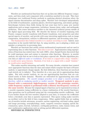
  • 7. AKUH· AMIN DAVAR , Fall-1390, WSP 7 Time Frequency Figure 1: Better time resolution Example Using the following sample signal x(t) that is composed of a set of four sinusoidal waveforms joined together in sequence. Each waveform is only composed of one of four frequencies (10, 25, 50, 100 Hz). The definition of x(t) is: x(t) =        cos(2π10t), cos(2π25t), cos(2π50t), cos(2π100t), N=400; t1=linspace(0,1,N); s1=cos(2*pi*10*t1);s2=cos(2*pi*20*t1);s3=cos(2*pi*40*t1);s4=cos(2*pi*80*t1); plot(t1,s1,t1+1,s2,t1+2,s3,t1+3,s4) plot(linspace(-200,200,4*400),abs(fftshift(fft([s1 s2 s3 s4])))); grid; figure(gcf) Let’s determine the spectral behavior using FFT plot(linspace(-200,200,4*400),abs(fftshift(fft([s1 s2 s3 s4])))); grid; figure(gcf) From figure 3, as we observe, there is no information as to the spectral behavior of sinusoidal signals(how many? what frequencies?). On the other hand, from figure 4, there is no information as to the beginning and end of each sinusoids though the frequencies are determined. In figure 6 we observe that each signal there is only one specific frequency centered around (10,20,40,80) for all times.
  • 8. AKUH· AMIN DAVAR , Fall-1390, WSP 8 Time Frequency Figure 2: Better frequency resolution subplot(221); spectrogram([s1],’’,0,256,400);title(’a’); figure(gcf) subplot(222); spectrogram([s2],’’,0,256,400);title(’b’); figure(gcf) subplot(223); spectrogram([s3],’’,0,256,400);title(’c’); figure(gcf) subplot(224); spectrogram([s4],’’,0,256,400);title(’d’); figure(gcf) Concatenation of the four sinusoids in time and frequency are distinguished using spectrogram([s1 s2 s3 s4],’’,0,256,400); figure(gcf) In mathematics, a wavelet series is a representation of a square-integrable (real- or complex-valued) function by a certain orthonormal series generated by a wavelet. A function ψ ∈ L2 (R) is called an orthonormal wavelet if it can be used to define a Hilbert basis, that is a complete orthonormal system, for the Hilbert space L2 (R) of square integrable functions. The Hilbert basis is constructed as the family of functions {ψjk : j, k ∈ Z} by means of dyadic translations and dilations of ψ, ψjk(x) = 2j/2 ψ(2j x − k) for integers j, k ∈ Z. This family is an orthonormal system if it is orthonormal under the inner product hψjk, ψlmi = δjlδkm where δjl is the Kronecker delta and hf, gi is the standard inner product hf, gi = R ∞ −∞ f(x)g(x)dx on L2 (R). The requirement of completeness is that every function f ∈ L2 (R) may be ex- panded in the basis as f(x) = ∞ X j,k=−∞ cjkψjk(x)
  • 9. AKUH· AMIN DAVAR , Fall-1390, WSP 9 0 0.5 1 1.5 2 2.5 3 3.5 4 −1 −0.8 −0.6 −0.4 −0.2 0 0.2 0.4 0.6 0.8 1 Time, sec. Figure 3: Concatenation of some sinusoids in time domain. −200 −150 −100 −50 0 50 100 150 200 0 50 100 150 200 250 freq., Hz Figure 4: Spectral behavior of concatenation of the sinusoids in frequency domain.
  • 10. AKUH· AMIN DAVAR , Fall-1390, WSP 10 0 50 100 150 200 0.2 0.4 0.6 0.8 Frequency (Hz) a Time 0 50 100 150 200 0.2 0.4 0.6 0.8 Frequency (Hz) b Time 0 50 100 150 200 0.2 0.4 0.6 0.8 Frequency (Hz) c Time 0 50 100 150 200 0.2 0.4 0.6 0.8 Frequency (Hz) d Time Figure 5: Time-frequency analysis of each individual sinusoids. 0 50 100 150 200 0.5 1 1.5 2 2.5 3 3.5 Frequency (Hz) Time Figure 6: Time-frequency analysis four concatenated sinusoids.
  • 11. AKUH· AMIN DAVAR , Fall-1390, WSP 11 Time Frequency Figure 7: Fourier basis functions, time-frequency tiles, and coverage of the time-frequency plane with convergence of the series understood to be convergence in norm. Such a repre- sentation of a function f is known as a wavelet series. This implies that an orthonormal wavelet is self-dual. The integral wavelet transform is the integral transform defined as [Wψf] (a, b) = 1 p |a| Z ∞ −∞ ψ x − b a f(x)dx The wavelet coefficients cjk are then given by cjk = [Wψf] (2j , k2j ) Here, a = 2j is called the binary dilation or dyadic dilation, and b = k2j is the binary or dyadic position. Introduction to the world of transform A mathematical operation that takes a function or sequence and maps into another one f(x) = Z F(w)K(w, x)dw
  • 12. AKUH· AMIN DAVAR , Fall-1390, WSP 12 fj = X j KijFi Examples: Laplace, Fourier, DTFT, DFT, FFT, z-transform Fourier Transform X(f) = Z ∞ −∞ x(t)e−2jπft dt x(t) = Z ∞ −∞ X(f)e2jπft df Fourier transform identifies all spectral components present in the signal, however it does not provide any information regarding the temporal (time) localization of the components. Fourier Transform : Limitations 1. Signals are of two types (a) Stationary (b) Non-stationary 2. Non-stationary signals are those who have got time varying spectral components . . . FT gives only provides the existence of the spectral components of the signal . . . But does not provide any information on the time occurrence of spectral compo- nents 3. The basis function e−jωt stretches to infinity, Hence, only analyzes the signal globally. 4. In order to obtain time-localization of spectral components, the signal need to be analyzed locally. Time–Frequency Representation 1. Instantaneous frequency: fx(t) = 1 2π d dt ∠x(t) 2. Group delay: tx(f) = − 1 2π d df ∠X(f) 3. Disadvantages of above expressions: These equations though have a huge theoretical significance but are not easy to implement. 4. All time-frequency-energy representations should be classified as time-frequency analysis; thus, wavelet, Wigner-Ville Distribution and spectrogram should all be included.
  • 13. AKUH· AMIN DAVAR , Fall-1390, WSP 13 5. Almost by default, the term, time-frequency analysis, was monopolized by the Wigner-Ville distribution. 6. To have a valid time-frequency representation, we have to have frequency and energy functions varying with time. Therefore, the frequency and energy functions should have instantaneous values Wigner-Ville Distribution Wigner-Ville Distribution, W(ω, t), is defined as W(ω, t) = 1 2π Z ∞ −∞ x(t − τ/2)x(t + τ/2) e−jωτ dτ E{W(ω, t)} = 1 2π Z ∞ −∞ E{x(t)x(t + τ)} e−jωτ dτ = 1 2π Z ∞ −∞ Rxx(t, τ) e−jωτ dτ WV Instantaneous Frequency ω(t) = R ∞ −∞ ωW(ω, t) dω R ∞ −∞ W(ω, t) dω 7. Therefore, at any given time, there is only one instantaneous frequency value. 8. What if there are two independent components? In this case, VW gives the weighted mean. If x(t) = x1(t) + x2 (t) then S(ω) = S1(ω) + S2(ω) , where S(ω) = 1 √ 2π R t x(t) e−iωt d t . |S|2 = |S1 + S2|2 = |S1|2 + |S2|2 + 2ℜ [S∗ 1S2] 6= |S1|2 + |S2|2 . Short-time Fourier Transform STFTw x (τ, w) = Z t [x(t)w(t − τ)]e−jwt dt
  • 14. AKUH· AMIN DAVAR , Fall-1390, WSP 14 • w(t) : windowing function generally a Gaussian pulse is used, other choices are rectangular, elliptic etc . . . • Maps 1D function to 2D time-frequency domain • Advantages: – Gives us time-frequency description of the signal – Overcomes the difficulties of Fourier transform by use of windowing functions STFT: Disadvantages • Heisenberg Principle: One can not get infinite time and frequency resolution beyond Heisenberg’s Limit ∆t ∆f ≥ 1 4π , ♣ where ∆t = sR ∞ −∞ t2|g(t)|2dt R ∞ −∞ |g(t)|2dt , ∆f = sR ∞ −∞ f2|G(f)|2df R ∞ −∞ |G(f)|2df Proof using Schwartz inequality: Z ∞ −∞ g1(s)g2(s)ds 2 ≤ Z ∞ −∞ g2 1(u)du Z ∞ −∞ g2 2(u)du Let’s g1(t) = tg(t), g2(t) = g′ (t) ⇒ Z ∞ −∞ tg(t)g′ (t)dt 2 ≤ Z ∞ −∞ t2 g2 (t)dt Z ∞ −∞ [g′ (t)]2 dt [g′ (t)]2 F ←→[j2πfG(f)] ∗ [j2πfG(f)] = −4π2 Z ∞ −∞ νG(ν)(f − ν)G(f − ν)dν ⇒ Z ∞ −∞ [g′ (t)]2 dt = 4π2 Z ∞ −∞ ν2 |G(ν)|2 dν g2 (t) F ←→ G(f) ∗ G(f) 2g′ (t)g(t) F ←→ j2πf[G(f) ∗ G(f)] Z ∞ −∞ g(t)g′ (t)e−j2πft dt = jπf Z ∞ −∞ G(ν)G(f − ν)dν ⇒ Z ∞ −∞ (−j2πt)g(t)g′ (t) e−j2πft
  • 15.
  • 16. f=0 dt = jπ Z ∞ −∞ G(ν)G(f − ν)
  • 17.
  • 18.
  • 19.
  • 21.
  • 22.
  • 23.
  • 24. f=0 −2 Z ∞ −∞ tg(t)g′ (t)dt = Z ∞ −∞ G(ν)G(−ν)dν = Z ∞ −∞ |G(f)|2 df
  • 25. AKUH· AMIN DAVAR , Fall-1390, WSP 15 −2 Z ∞ −∞ tg(t)g′ (t)dt = Z ∞ −∞ |G(f)|2 df Z ∞ −∞ tg(t)g′ (t)dt 2 ≤ Z ∞ −∞ t2 g2 (t)dt Z ∞ −∞ 4π2 f2 |G(f)|2 df Divide both sides by E2 g = Z ∞ −∞ g2 (t)dt 2 = Z ∞ −∞ |G(f)|2 df 2 to have the desired result ♣. The function that satisfies ♣ with equality is Gaussian: g1(t) = K0g2(t) ⇒ tg(t) = K0g′ (t) ⇒ g(t) = K1et2/K0 • Trade offs: – Wider window: Good frequency resolution, Poor time resolution – Narrower window: Good time resolution, Poor frequency resolution The definition of the class of bilinear (or quadratic) time-frequency distributions: Cx(t, f) = Z ∞ −∞ Z ∞ −∞ Ax(η, τ)Φ(η, τ) exp(−j2π(ηt + τf)) dη dτ, where Ax (η, τ) is the ambiguity function . Φ (η, τ) is the kernel function which is usually a low-pass function and is used to mask out the interference. The class of bilinear (or quadratic) time-frequency distributions can be most easily understood in terms of the ambiguity function an explanation of which follows. Consider the well known power spectral density Px (f) and the signal auto-correlation function Rx (τ) in the case of a stationary process. The relationship between these Px(f) = Z ∞ −∞ Rx(τ)ej2πfτ dτ, (4) Rx(τ) = E{x(t + τ/2)x∗ (t − τ/2)} (5) For a non-stationary signal x (t) , these relations can be generalized using a time-dependent power spectral density or equivalently the famous Wigner distribution function of x (t) as follows: Wx(t, f) = Z ∞ −∞ Rx(t, τ)e−j2πfτ dτ, (6) Rx (t, τ) = E{x(t + τ/2)x(t − τ/2)}. (7) If the Fourier transform of the auto-correlation function is taken with respect to t instead of τ, we get the ambiguity function as follows: Ax(η, τ) = Z ∞ −∞ x(t + τ/2)x∗ (t − τ/2)ej2πtη dt.
  • 26. AKUH· AMIN DAVAR , Fall-1390, WSP 16 Ax(η, τ) FtF−1 f Fτ F−1 η Wx(t, f) Rx(t, τ) Ft F−1 η F−1 f Fτ Figure 8: The relationship between the Wigner distribution function, the auto- correlation function and the ambiguity function. Linear vs. Quadratic Distributions Linear: Quadratic Pros: Pros: Linear superposition Better time and frequency resolutions than linear No interference terms for muti-component signals Shows the energy distribution Cons: Cons: Trade off between time and frequency resolutions Cross terms for multi-component signals Heisenberg inequality Wavelet Transform • Overcomes the shortcoming of STFT by using variable length windows: i.e. Nar- rower window for high frequency thereby giving better time resolution and Wider window at low frequency thereby giving better frequency resolution • Heisenberg’s Principle still holds • Mathematical formula: CWTΨ x (τ, s) = Ψ(τ, s) = 1 p |s| Z t x(t)Ψ∗ ( t − τ s )dt where
  • 27. AKUH· AMIN DAVAR , Fall-1390, WSP 17 Absolute Values of Ca,b Coefficients for a = 0.01 1.02 2.03 3.04 4.05 ... time (or space) b scales a 100 200 300 400 500 600 0.01 5.06 10.11 15.16 20.21 25.26 30.31 35.36 40.41 45.46 50.51 55.56 60.61 65.66 70.71 75.76 80.81 85.86 90.91 95.96 50 100 150 200 Figure 9: Continuous wavelet of δ(t) for small scales(large frequencies) around 400 are strong and as we move away from b = 400 there is conic relationship between scales and delays. x(t) = given signal τ = translation parameter s = scaling parameter = 1/f Ψ(t) = Mother wavelet , All kernels are obtained by scaling and/or translating mother wavelet Example using Morlet wavelet Ψ(t) = cos(5t)e−t2/2 : x=[zeros(1,400) 1 zeros(1,199)]; s=cwt(x,linspace(1e-2,100,100),’morl’,’plot’); figure(gcf);pause; colormap(’default’); X=linspace(0,100,100);Y=0:599; contour(Y,X,s);figure(gcf);pause; mesh(Y,X,s);figure(gcf) x=cos(2*pi*5*(0:199)/200); s=cwt(x,linspace(1e-2,50,100),’morl’,’plot’); figure(gcf);pause;colormap(’default’); X=linspace(1e-2,50,100);Y=0:199;contour(Y,X,s); figure(gcf);pause; mesh(Y,X,s);figure(gcf)
  • 28. AKUH· AMIN DAVAR , Fall-1390, WSP 18 0 100 200 300 400 500 0 10 20 30 40 50 60 70 80 90 100 −0.4 −0.3 −0.2 −0.1 0 0.1 0.2 0.3 0.4 Figure 10: Contour plot of wavelet of δ(t), for scales less than 30 wavelet vales of δ(t) are large around b = 400. Figure 11: Mesh plot of wavelet of δ(t).
  • 29. AKUH· AMIN DAVAR , Fall-1390, WSP 19 Absolute Values of Ca,b Coefficients for a = 0.01 0.51495 1.0199 1.5248 2.0298 ... time (or space) b scales a 50 100 150 200 0.01 2.53475 5.05949 7.58424 10.109 12.6337 15.1585 17.6832 20.208 22.7327 25.2575 27.7822 30.307 32.8317 35.3565 37.8812 40.406 42.9307 45.4555 47.9802 50 100 150 200 Figure 12: Continuous wavelet of cos(2π5t) for small scales around 30 for almost all delays is strong but we observe some repetition in x−axis. 0 50 100 150 5 10 15 20 25 30 35 40 45 50 −6 −4 −2 0 2 4 6 Figure 13: Contour plot of wavelet of cos(2π5t), for scales around 30 wavelet vales of δ(t) are strong.
  • 30. AKUH· AMIN DAVAR , Fall-1390, WSP 20 0 50 100 150 200 0 20 40 60 −10 −5 0 5 10 −6 −4 −2 0 2 4 6 Figure 14: Mesh plot of wavelet of cos(2π5t). close all t=linspace(0,1,100); x=[sin(2*pi*5*t)]; figure(1) cw1 = cwt(x,1:30,’morl’,’plot’); title(’Continuous Transform, absolute coefficients.’) ylabel(’Scale’) figure(2) %[cw1,sc] = cwt(x,1:40,’morl’,’scal’); [cw1,sc] = cwt(x,1:30,’morl’,’scalCNT’); title(’Scalogram’) ylabel(’Scale’) figure(gcf) close all t=linspace(0,1,100); x=[sin(2*pi*5*t) sin(2*pi*15*t) sin(2*pi*25*t)]; figure(1) cw1 = cwt(x,1:30,’morl’,’plot’); title(’Continuous Transform, absolute coefficients.’) ylabel(’Scale’) figure(2) %[cw1,sc] = cwt(x,1:40,’morl’,’scal’); [cw1,sc] = cwt(x,1:30,’morl’,’scalCNT’); title(’Scalogram’)
  • 31. AKUH· AMIN DAVAR , Fall-1390, WSP 21 ylabel(’Scale’) figure(gcf) Scale values determine the degree to which the wavelet is compressed or stretched. Low scale values compress the wavelet and correlate better with high frequencies. The low scale CWT coefficients represent the fine-scale features in the input signal vector. High scale values stretch the wavelet and correlate better with the low frequency content of the signal. The high scale CWT coefficients represent the coarse-scale features in the input signal. Continuous Wavelet transform • The kernel functions used in wavelet transform are all obtained from one prototype function known as mother wavelet, by scaling and/or translating it. Ψa,b(t) = 1 √ a Ψ( t − b a ) a = scale parameter b = translation parameter Ψ1,0(t) = Ψ(t) • Continuous Wavelet transform W(a, b) = 1 √ a Z ∞ −∞ x(t)Ψa,b(t)dt • In order to become a wavelet a function must satisfy the above two conditions Z ∞ −∞ Ψ(t)dt = 0 Z ∞ −∞ |Ψ(t)|2 dt ∞ Inverse wavelet transform x(t) = 1 C Z ∞ −∞ Z ∞ −∞ 1 a2 W(a, b)Ψa,b(t)dadb where C = Z ∞ −∞ |Ψ(w)| |w| dw provided Z ∞ −∞ Ψ(t)dt = 0
  • 32. AKUH· AMIN DAVAR , Fall-1390, WSP 22 Proof: f(ω) = 1 2π Z ∞ −∞ f(t)e−jωt dt, Fourier transform F(ω, s) = 1 2π Z ∞ −∞ f(t)g(t − s)e−jωt dt, Windowed transform For each s, we recover f(t)g(t − s) by f(t)g(t − s) = Z ∞ −∞ F(ω, s)ejωt dω Multiply both sides by g∗ (t − s) and integrate over s. f(t) Z ∞ −∞ g(t − s)g∗ (t − s)ds = Z ∞ −∞ Z ∞ −∞ F(ω, s)g∗ (t − s)ejωt dωds f(t) = 1 ||g(t)||2 Z ∞ −∞ Z ∞ −∞ F(ω, s)g∗ (t − s)ejωt dωds This is the reconstruction from time-frequency(space) transform. So far we concentrated on windowed STFT. Wavelets begin with one function Ψ(t). The position variable s still comes from translation Ψ(t − s). Now comes the difference. Instead of the frequency variable we have a scale variable. Instead of modulating them we rescale them. The “time-scale atoms” are the translates and dilates of Ψ(t) : Ψa,b(t) = 1 √ a Ψ((t − b)/a), Wavelet functions The mother wavelet is Ψ(t) = Ψ1,0(t). The factor |a|−0.5 assures that rescaled wavelets have equal energy ||Ψa,b(t)|| = ||Ψ(t)||. We normalize so that all these functions have unit norm ||Ψa,b(t)|| = 1. Scaling the time by aj automatically scales the translation steps by a−j Ψ(aj t − k) = Ψ(aj [t − a−j k]) The mesh length at level j is scaled down by a−j . The frequency is scaled up by aj . This hyperbolic scaling or dyadic scaling or octave scaling (a = 2) is a prime characteristic of wavelet analysis. Any smooth decaying function Ψ(t) is a mother wavelet provided that Z Ψ(t)dt = 0 F n Wf (a, b) = f(t) ∗ p |a|−1Ψ(−t/a) o = p |a|F(ω)Ψ∗ (aω)
  • 33. AKUH· AMIN DAVAR , Fall-1390, WSP 23 F nh Wg(a, b) = g(t) ∗ p |a|−1Ψ(−t/a) i∗o = p |a|G∗ (ω)Ψ(aω) Wf (a, b) ←→ p |a|F(ω)Ψ∗ (aω) W∗ g (a, b) ←→ p |a|G(ω)Ψ(aω) Multiply Wf (a, b) and W∗ g (a, b) and integrate over b Z ∞ −∞ Wf (a, b)W∗ g (a, b)db = 2π Z ∞ −∞ |a|F(ω)G∗ (ω)|Ψ(aω)|2 dω Integrate this equation with respect to da/|a|2 and reverse the order of integration: Z ∞ −∞ Z ∞ −∞ Wf (a, b)W∗ g (a, b) dadb |a|2 = 2π Z ∞ −∞ Z ∞ −∞ |a|F(ω)G∗ (ω)|Ψ(aω)|2 dωda |a|2 , U 2π Z ∞ −∞ Z ∞ −∞ F(ω)G∗ (ω)|Ψ(aω)|2 dωda |a| = 2π Z ∞ −∞ F(ω)G∗ (ω)dω Z ∞ −∞ |Ψ(aω)|2 da |a| 2π Z ∞ −∞ |Ψ(aω)|2 da |a| = 2π Z ∞ −∞ |Ψ(ω)|2 |ω| dω Obtained by ν = aω, dν = ωda, da/|a| = dω/|ω| Therefore, Z ∞ −∞ Z ∞ −∞ Wf (a, b)W∗ g (a, b) dadb |a|2 = C Z ∞ −∞ f(t)g∗ (t)dt, C = 2π Z ∞ −∞ |Ψ(ω)|2 |ω| dω By assuming g(t − τ) = δ(t) ⇒ Wg(a, b) = Ψ((τ − b)/a)/ √ a, from equation U we have Z ∞ −∞ Z ∞ −∞ Wf (a, b)Ψ((τ − b)/a)/ √ a dadb |a|2 = C Z ∞ −∞ f(t)δ(t − τ)dt = Cf(τ) ⇒ f(t) = 1 C Z ∞ −∞ Z ∞ −∞ Wf (a, b)Ψ((t − b)/a)/ √ a dadb |a|2 Example of Meyer wavelet and its Fourier transform Meyer wavelet is defined in frequency domain, by refering to MATLAB for their representation: ψ(ω) = ( ejω/2 √ 2π sin(0.5v(3|ω|/2π − 1)) 2π 3 ≤ |ω| ≤ 4π 3 ejω/2 √ 2π sin(0.5v(3|ω|/4π − 1)) 4π 3 ≤ |ω| ≤ 8π 3 ψ(ω) = 0, ω ∋ 2π 3 , 8π 3 v(a) = a4 (35 − 84a + 70a2 − 20a3 ), a ∈ [0, 1] φ(x) = 1 √ 2π |ω| ≤ 2π 3 φ(x) = 1 √ 2π cos(0.5v(3|ω|/2/π − 1)) 2π 3 ≤ |ω| ≤ 4π 3 φ(x) = 0 |ω| ≥ 4π 3
  • 34. AKUH· AMIN DAVAR , Fall-1390, WSP 24 −8 −6 −4 −2 0 2 4 6 8 −1 −0.5 0 0.5 1 1.5 Meyer wavelet: ψ(x) x ψ(x) −600 −400 −200 0 200 400 600 −200 −150 −100 −50 0 50 f F{ψ(x)} Figure 15: Wavelet ψ and its Fourier transform, they are very much concentrated in time and frequency domain. [phi,psi,x] = wavefun(’meyr’,10); figure(1) subplot(211) plot(x,psi);grid;figure(gcf); title(’Meyer wavelet: $psi(x)$’) xlabel(’$x$’);ylabel(’$psi(x)$’); subplot(212) f=linspace(-.5,.5,length(x))*length(x); PSI=abs(fftshift(fft(psi))); plot(f,10*log10(PSI));grid;figure(gcf); xlabel(’$f$’);ylabel(’$mathcal{F}{psi(x)}$’); figure(2) subplot(211) plot(x,phi);grid;figure(gcf); title(’Meyer wavelet: $phi(x)$’) xlabel(’$x$’);ylabel(’$phi(x)$’); subplot(212) f=linspace(-.5,.5,length(x))*length(x); PHI=abs(fftshift(fft(phi))); plot(f,10*log10(PHI));grid;figure(gcf); xlabel(’$f$’);ylabel(’$mathcal{F}{phi(x)}$’);
  • 35. AKUH· AMIN DAVAR , Fall-1390, WSP 25 −8 −6 −4 −2 0 2 4 6 8 −0.5 0 0.5 1 1.5 Meyerwavelet: φ(x) x φ(x) −600 −400 −200 0 200 400 600 −200 −100 0 100 f F {φ(x)} Figure 16: Scaling function(father wavelet) φ and its Fourier transform, they are very much concentrated in time and frequency domain. Constant Q-filtering • CWT can be rewritten as W(a, b) = x(b) ∗ Ψ∗ a,0(−b) Proof: Ψa,0(t) = 1 √ a Ψ(t/a) ⇒ Ψa,0(−b) = 1 √ a Ψ(−b/a) x(b) ∗ Ψa,0(−b) = Z ∞ −∞ x(t) 1 √ a Ψ(−(b − t)/a) = CWTΨ x (a, b) • A special property of the above filter defined by the mother wavelet is that they are Constant-Q filters • Q factor = Center frequency/Bandwidth Q = 2π Energy Stored Energy dissipated per cycle = 2πfr Energy Stored Power Loss , fr = resonant frequency • Hence the filter defined by wavelet increases their Bandwidth as scale increases ( i.e. center frequency increases ) • This leads to filter bank implementation of discrete wavelet transform
  • 36. AKUH· AMIN DAVAR , Fall-1390, WSP 26 I. Daubechies believes that the wavelet transform can be used to analyze time series that contain nonstationary power at many different frequencies. The term “wavelet function” is used generically to refer to either orthogonal or nonorthogonal wavelets. The term “wavelet basis” refers only to an orthogonal set of functions. The use of an orthogonal basis implies the use of the discrete wavelet transform, while a nonorthogonal wavelet function can be used with either the discrete or the continuous wavelet transform. The continuous wavelet transform of a discrete sequence xn is defined as the convolution of xn with a scaled and translated version of ψ0(t): Wn(s) = N−1 X n′=0 xn′ ψ∗ ((n′ − n)δt/s) (8) in this formula ψ(·) is normalized: Z ∞ −∞ |ψ̂(ω′ )|2 dω′ = 1 Use of DFT allows to do convolution (8) easily x̂k = 1 N N−1 X n=0 xne−j2πkn/N Using F{ψ(t/s)} = ψ̂(sω), By the convolution theorem, the wavelet transform is the inverse Fourier transform of the product: Wn(s) = N−1 X k=0 x̂kψ̂∗ (sωk)ejωknδt (9) angular frequency ωk : ωk =        2πk Nδt , k ≤ N − 2πk Nδt , k N Using (9), the continuous wavelet transform (for a given s) at all n is calculated simultaneously and efficiently. To ensure that the wavelet transforms (9) at each scale s are directly comparable to each other and to the transforms of other time series, the wavelet function at each scale s is normalized to have unit energy: ψ̂(sωk) = r 2πs δt ψ̂0(sωk), ψ((n′ − n)δt/s) = r δt s ψ((n′ − n)δt/s) (10)
  • 37. AKUH· AMIN DAVAR , Fall-1390, WSP 27 Name ψ0(t) ψ̂0(sω) Morlet (ω0=frequency) π−1/4 ejω0t e−t2/2 π−1/4 H(ω)e−(sω−ω0)2/2 Paul (m=order) 2mjmm! √ π(2m)! (1 − jt)−(m+1) 2m √ m(2m−1)! H(ω)(sω)m e−sω DOG (m=derivative) (−1)m+1 √ Γ(m+1/2) dm dtm e−t2/2 −jm √ Γ(m+1/2) (sω)m e−(sω)2/2 Table 1: H(ω) = Heaviside step function, H(ω) = 1 if ω 0, H(ω) = 0 otherwise. DOG = derivative of a Gaussian; m = 2 is the Marr or Mexican hat wavelet. Some of the unscaled ψ̂0 are defined in Table 1 to have Z ∞ −∞ |ψ̂(ω′ )|2 dω′ = 1 Using these normalizations, at each scale s : N−1 X k=0 |ψ̂(sωk)|2 = N Discrete wavelet Transform • Discrete domain counterpart of CWT • Implemented using Filter banks satisfying PR(perfect reconstruction) condition • Represents the given signal by discrete coefficients {dk,n} • DWT is given by Ψk,n(t) = 2−k/2 Ψ(2−k t − n) x(t) = X k X n dk,nΨk,n(t), dk,n = hx, Ψk,ni = Z x(t)Ψ∗ k,n(t)dt Scaling Function • These are functions used to approximate the signal up to a particular level of detail φk,n(t) = 2k/2 φ(2k t − n)
  • 38. AKUH· AMIN DAVAR , Fall-1390, WSP 28 0 0.5 1 0 0.5 1 1.5 t Φ(t) 0 0.5 1 −2 −1 0 1 2 Ψ(t) t Figure 17: Haar Scaling and Wavelet Function. [PHI,PSI,XVAL] = wavefun(’db2’,9) f=linspace(-.5,.5,length(XVAL))*length(XVAL) G1=abs(fftshift(fft(PSI))); G2=abs(fftshift(fft(PSI))); Refinement equation and wavelet Equation • Refinement equation is an equation relating to scaling function and filter coefficients φ(t) = √ 2 N X k=0 h0(k)φ(2t − k), h0(k) is even length, X k h0(k) = √ 2 • Wavelet equation is an equation relating to wavelet function and filter coefficients ψ(t) = 2 N X k=0 h1(k)ψ(2t − k) • By solving the above two we can obtain the scaling and wavelet function for a given filter bank structure Some Important properties of wavelets • Compact Support: – Finite duration wavelets are called compactly supported in time domain but are not band-limited in frequency. They can be implemented using FIR filters – Examples: Haar, Daubechies, Symlets , Coiflets – Narrow band wavelets are called compactly supported in frequency domain. Can be implemented using IIR filters
  • 39. AKUH· AMIN DAVAR , Fall-1390, WSP 29 0 1 2 3 −0.5 0 0.5 1 1.5 t Φ(t) 0 1 2 3 −2 −1 0 1 2 t Ψ(t) −1000 0 1000 −60 −40 −20 0 f 10log 10 (F {Φ(t)}) −1000 0 1000 −200 −150 −100 −50 0 f 10log 10 (F {Ψ(t)}) Figure 18: Db2 Scaling and Wavelet Function. – Examples: Meyer’s wavelet • Symmetry • Symmetric / Antisymmetric wavelets have linear-phase • Orthogonal wavelets are asymmetric and have a non-linear phase • Biorthogonal wavelets are asymmetric but have linear phase and can be implemented using FIR filters • Vanishing Moment: R tk ψ(t)dt = 0, k = 0, 1, · · · , p − 1 • p-th vanishing moment is defined as Mp = Z tp Ψ(t)dt • The more the number of moments of a wavelets are zero the more is its compressive power • Smoothness • it is roughly the number of times a function can be differentiated at any given point • This is closely related to vanishing Moments • Smoothness provides better numerical stability
  • 40. AKUH· AMIN DAVAR , Fall-1390, WSP 30 • It also provides better reconstruction property Orthogonal wavelet An orthogonal wavelet is a wavelet where the associated wavelet transform is orthogonal. That is the inverse wavelet transform is the adjoint of the wavelet transform. If this condition is weakened you may end up with biorthogonal wavelets. Orthogonal filters using MATLAB: [H0,H1,F0,F1] = wfilters(’db2’) sum(H0.*H1)=-6.9389e-018 sum(F0.*F1)= 6.9389e-018 Biorthogonal filters using MATLAB: [Rf,Df] = biorwavf(’bior3.3’) 8 filters are obtained: [H01,H11,F01,F11,H02,H12,F02,F12] = biorfilt(Df,Rf,’8’) sum(H01.*H11)=1.0495e-016 sum(F01.*F11)=-1.0495e-016 sum(H02.*H12)=6.9389e-018 sum(F02.*F12)=-6.9389e-018 The scaling function is a refinable function. That is, it is the a fractal functional equation, called refinement equation: φ(x) = N−1 X k=0 akφ(2x − k), where the sequence (a0, . . . , aN−1) of real numbers is called scaling sequence or scaling mask. The wavelet proper is obtained by a similar linear combination, ψ(x) = M−1 X k=0 bkφ(2x − k), where the sequence (b0, . . . , bM−1) of real numbers is called wavelet sequence or wavelet mask.
  • 41. AKUH· AMIN DAVAR , Fall-1390, WSP 31 A necessary condition for the orthogonality of the wavelets is, that the scaling sequence is orthogonal to any shifts of it by an even number of coefficients: X n∈Z anan+2m = 2δm,0 X (−1)k km h0(k) = 0, m = 0, 1, · · · , p − 1 In this case there is the same number M=N of coefficients in the scaling as in the wavelet sequence, the wavelet sequence can be determined as bn = (−1)n aN−1−n. In some cases the opposite sign is chosen. Vanishing moments, polynomial approximation and smoothness A necessary condition for the existence of a solution to the refinement equation is, that some power (1 + Z)A , A 0, divides the polynomial a(Z) := a0 + a1Z + · · · + aN−1ZN−1 . The maximally possible power A is called polynomial approximation order (or pol. app. power) or number of vanishing moments. It describes the ability to represent polynomials up to degree A − 1 with linear combinations of integer translates of the scaling function. In the biorthogonal case, an approximation order A of φ corresponds to A vanishing moments of the dual wavelet ψ̃, that is, the scalar products of ψ̃ with any polynomial up to degree A − 1 are zero. In the opposite direction, the approximation order à of φ̃ is equivalent to à vanishing moments of ψ. In the orthogonal case, A and à coincide. Biorthogonal filters using MATLAB can have linear phase [PHI1,PSI1,PHI2,PSI2,XVAL] = wavefun(’bior3.3’,5); plot(XVAL,abs(fftshift(fft(PSI1))),XVAL,abs(fftshift(fft(PSI2)))) plot(XVAL,angle(fft(PSI1)),XVAL,angle(fft(PSI2))) A sufficient condition for the existence of a scaling function is the following: If one decomposes a(Z) = 21−A (1 + Z)A p(Z), and the estimate holds 1 ≤ sup t∈[0,2π] |p(eit )| 2A−1−n for some n ∈ N, holds, then the refinement equation has a n times continuously differentiable solution with compact support. Examples:
  • 42. AKUH· AMIN DAVAR , Fall-1390, WSP 32 • a(Z) = 21−A (1+Z)A , that is p(Z) = 1, has n = A−2. The solutions are Schoenbergs B-splines of order A − 1, where the (A − 1)-th derivative is piecewise constant, thus the (A − 2)-th derivative is Lipschitz-continuous. A = 1 corresponds to the index function of the unit interval. • A = 2 and p linear may be written as a(Z) = 1 4 (1 + Z)2 ((1 + Z) + c(1 − Z)). Expansion of this degree 3 polynomial and insertion of the 4 coefficients into the orthogonality condition results in c2 = 3. The positive root gives the scaling sequence of the Db4-wavelet. Biorthogonal wavelet A biorthogonal wavelet is a wavelet where the associated wavelet transform is invertible but not necessarily orthogonal. Designing biorthogonal wavelets allows more degrees of freedoms than orthogonal wavelets. One additional degree of freedom is the possibility to construct symmetric wavelet functions. In the biorthogonal case, there are two scaling functions φ, φ̃, which may generate different multiresolution analyses, and accordingly two different wavelet functions ψ, ψ̃. So the numbers M, N of coefficients in the scaling sequences a, ã may differ. The scaling sequences must satisfy the following biorthogonality condition X n∈Z anãn+2m = 2 δm,0. Then the wavelet sequences can be determined as bn = (−1)n ãM−1−n, n = 0, . . . , M − 1 and b̃n = (−1)n aM−1−n, n = 0, . . . , N − 1. Down-Sampling: y[n] = x[2n]        . . . y[−1] y[0] y[1] . . .        =       · · · · · · · · · · · · · · · · · · · · · · · · 1 0 0 0 0 · · · · · · 0 0 1 0 0 · · · · · · 0 0 0 0 1 · · · · · · · · · · · · · · · · · · · · · · · ·                . . . x[−1] x[0] x[1] x[2] . . .         
  • 43. AKUH· AMIN DAVAR , Fall-1390, WSP 33 Y (ejω ) = 1 2 X ejω/2 + X ej(ω−2π)/2 Y (z) = 1 2 X z1/2 + X −z1/2 Up-Sampling: y[n] = x[n/2], n even 0, n odd          . . . y[−1] y[0] y[1] y[2] . . .          =           · · · · · · · · · · · · · · · · · · 1 0 0 · · · · · · 0 0 0 · · · · · · 0 1 0 · · · · · · 0 0 0 · · · · · · 0 0 1 · · · · · · · · · · · · · · · · · ·                    . . . x[−1] x[0] x[1] x[2] . . .          Y (ejω ) = X (ej2ω ) Y (z) = X (z2 ) Filter Bank(FB): First FB designed for speech coding, [Croisier-Esteban-Galand 1976] Orthogonal FIR filter bank, [Smith-Barnwell 1984], [Mintzer 1985] H0(z) H1(z) ↓ 2 ↓ 2 Q Q is processing ↑ 2 ↑ 2 F1(z) F0(z) + X̂(z) X(z) Figure 19: FB analysis and synthesis. Example using MATLAB x=[zeros(1,100) ones(1,100) zeros(1,100)]; [xa,xd]=dwt(x,’db2’); plot(xa);figure(gcf);pause plot(xd);figure(gcf);pause [xa,xd]=dwt(x,’bior3.3’); plot(xa);figure(gcf);pause plot(xd);figure(gcf);pause
  • 44. AKUH· AMIN DAVAR , Fall-1390, WSP 34 X̂(z) = 1 2 for Distortion Elimination, set to 2z−ℓ z }| { [F0(z)H0(z) + F1(z)H1(z)] X(z) + 1 2 [F0(z)H0(−z) + F1(z)H1(−z)] | {z } for Aliasing Cancellation, set to 0 X(−z) = z−ℓ X(z) The filters H0(z) and H1(z) are still to be chosen, these choices are connected. Historically, designers chose the lowpass filter coefficients {h0(0), · · · , h0(N)} and then construct H0(z) and H1(z). There are three possibilites that produce equal length filters: Early choice: Alternating signs: H1(z) = H0(−z) to produce h1(k) = {h0(0), −h0(1), h0(2), −h0(3) · · ·} Better choice: Alternating flip: H1(z) = −z−N H0(−z−1 ) to produce h1(k) = {h0(N), −h0(N − 1), · · ·} General choice: F0(z)H0(z) is a halfband filter. This gives biorthogonality, when aliasing is cancelled by relation of F0 to H0 and F1 to H1 Alternating-Sign Construction: F0(z) = H1(−z) F1(z) = −H0(−z) Perfect Reconstruction: With Aliasing Cancellation: F0(z) = H1(−z) F1(z) = −H0(−z) Distortion Elimination becomes: F0(z)H0(z) − F0(−z)H0(−z) = 2z−l Half-band Filter: ⇒ P0(z) − P0(−z) = 2z−ℓ where P0(z) ≡ F0(z)H0(z) Half-band Filter: P0(z) = a + bz−1 + cz−2 + dz−3 + ez−4 P0(−z) = a − bz−1 + cz−2 − dz−3 + ez−4
  • 45. AKUH· AMIN DAVAR , Fall-1390, WSP 35 P0(z) − P0(−z) = 0 + 2bz−1 + 0 + 2dz−3 + 0 = 2z−ℓ can only have one odd-power Standard design procedure: Design a good low-pass half-band filter P0(z) Factor P0(z) into H0(z) and F0(z) Use the aliasing cancellation condition to obtain H1(z) and F1(z) Examples: [H0,H1,F0,F1] = wfilters(’db2’) P0=conv(H0,F0)=[-0.0625,0.0000,0.5625,1.0000,0.5625,0.0000,-0.0625] [H W]=freqz(P0); HH=polyval(P0,exp(j*(W+pi))); plot(W,abs(H)/16,W,abs(HH)) Spectral Factorization: Orthogonality: fi[n] = hi[−n], Fi(z) = Hi(z−1 ) Example: [H0,H1,F0,F1] = wfilters(’db2’); f_i [n] = h_i [ - n]: H0 =[-0.1294,0.2241,0.8365,0.4830] F0=[0.4830,0.8365,0.2241,-0.1294] H1=[-0.4830,0.8365,-0.2241,-0.1294] F1=[-0.1294,-0.2241,0.8365,-0.4830] z and z−ℓ must be separated Symmetry: hi[n] = ±hi[L − 1 − n], Hi(z) = ±z−(L−1) Hi(z−1 ) z and z−ℓ must stay together P0(z) = H0(z)F0(z) = Y n (1 − znz−1 ); {zn} = roots H0(z) = Y k∈H (1 − zkz−1 ) F0(z) = Y ℓ∈F (1 − zℓz−1 ) Filter Banks(FB): perfect reconstruction; halfband filters and possible factorizations. Example: Product filter of degree 6
  • 46. AKUH· AMIN DAVAR , Fall-1390, WSP 36 multiple zeros at z = −1 ℜ(z) ℑ(z) Figure 20: Zeros of Half-band Filter. [H0,H1,F0,F1] = wfilters(’db2’); P0(z) = conv(H0, F0) = 1 16 (−1 + 9z−2 + 16z−3 + 9z−4 − z−6 ) P0(z) − P0(−z) = 2z−3 ⇒ Expect perfect reconstruction with a 3 sample delay Centered form: P(z) = z3 P0(z) = 1 16 (−z3 + 9z1 + 16 + 9z−1 − z−3 ) P(z) + P(−z) = 2 In the frequency domain: P(eiω ) + P(ei(ω+π) ) = 2, halfband condition
  • 47. AKUH· AMIN DAVAR , Fall-1390, WSP 37 ω Halfband π/2 1 Figure 21: Antisymmetry about ω = π/2. How do we factor P0(z) into H0(z)F0(z)? P0(z) = 1 16 (1 + z−1 )4 (−1 + 4z−1 − z−2 ) = − 1 16 (1 + z−1 )4 (2 + √ 3 − z−1 )(2 − √ 3 − z−1 )) 4th order zero at z = −1 ℜ(z) ℑ(z) Some possible factorizations: H0(z) or F0(z) F0(z) or H0(z) (a) 1 − 1 16 (1 + z−1)4(2 + √ 3 − z−1)(2 − √ 3 − z−1) (b) (1 + z−1 )/2 − 1 8 (1 + z−1 )3 (2 + √ 3 − z−1 )(2 − √ 3 − z−1 ) (c) (1 + z−1 )/4 − 1 4 (1 + z−1 )2 (2 + √ 3 − z−1 )(2 − √ 3 − z−1 ) (d) (1 + z−1 )(2 + √ 3 − z−1 )/2 − 1 8 (1 + z−1 )3 (2 − √ 3 − z−1 ) (e) (1 + z−1 )3 /8 − 1 2 (1 + z−1 )(2 + √ 3 − z−1 ))(2 − √ 3 − z−1 ) (f) √ 3−1 4 √ 2 (1 + z−1 )2 (2 + √ 3 − z−1 )) − √ 2 4( √ 3−1) (1 + z−1 )2 (2 − √ 3 − z−1 ) (g) 1 16 (1 + z−1 )4 (2 + √ 3 − z−1 )(2 − √ 3 − z−1 ) case (b)– Symmetric filters (linear phase): Case (c)–Symmetric filters (linear phase) Case (f)–Orthogonal filters (minimum phase/maximum phase) that, in this case, one filter is the flip (transpose) of the other: f0(n) = h0(3 − n) ⇔ F0(z) = z−3 H0(z−1 )
  • 48. AKUH· AMIN DAVAR , Fall-1390, WSP 38 1st order 2− √ 3 2+ √ 3 3rd order filter length=2 1/2{1, 1} filter length=6 1/4{−1, 1, 8, 8, 1, −1} 2nd order 2− √ 3 2+ √ 3 2nd order filter length=3 1/4{1, 2, 1} filter length=5 1/4{−1, 2, 6, 2, −1} General form of product filter (to be derived later): P(z) = 2 1 + z−1 2 p 1 + z 2 p p−1 X k=0 p + k − 1 k 1 − z 2 k 1 + z−1 2 k P0(z) = z−(2p−1) P(z) (11) = (1 + z−1 )2p | {z } Binomial (spline filter) 1 22p−1 p−1 X k=0 p + k − 1 k (−1)k z−(p−1)+k 1 − z−1 2 2k | {z } Q(z) cancels all odd powers except z−(2p−1) (12)
  • 49. AKUH· AMIN DAVAR , Fall-1390, WSP 39 2− √ 3 2nd order 2+ √ 3 2nd order filter length=4 1 4 √ 2 n 1 + √ 3, 3 + √ 3, 3 − √ 3, 1 − √ 3 o filter length=4 1 4 √ 2 n 1 − √ 3, 3 − √ 3, 3 + √ 3, 1 + √ 3 o p = 1 P0(z) has degree 2 99K leads to Haar filter bank. {1, 1, 1, 1} H0(z) H1(z) ↓2 ↓2 {0, 0} {1, 1} H0(z) H1(z) ↓2 ↓2 1 0 F0(z) = 1 + z−1 , H0(z) = 1+z−1 2 , H1(z) = 1 − z−1 Synthesis lowpass filter has 1 zero at π Leads to cancellation of constant signals in analysis highpass channel. Additional zeros at π would lead to cancellation of higher order polynomials.
  • 50. AKUH· AMIN DAVAR , Fall-1390, WSP 40 p = 2 P0(z) has degree 4p − 2 = 6 From (11): P0(z) = 1 16 (−1 + 9z−2 + 16z−3 + 9z−4 − z−6 ) Possible factorizations: {1/8, 2/6, 3/5 | {z } linear phase , 4/4 |{z} db4 } 2− √ 3 2+ √ 3 4nd order % function [p0,b,q] = prodfilt(p) % % Generate the halfband product filter of degree 4p-2. % % p0 = coefficients of product filter of degree 4p-2. % b = coefficients of binomial (spline) filter of degree 2p % q = coefficients of filter of degree 2p-2 that produces the halfband % filter p0 when convolved with b. function [p0,b,q] = prodfilt(p) % Binomial filter (1 + z^-1)^2p tmp1 = [1 1]; b = 1; for k = 0:2*p-1 b = conv(b, tmp1); end % Q(z) tmp2 = [-1 2 -1] / 4; q = zeros(1,2*p-1);
  • 51. AKUH· AMIN DAVAR , Fall-1390, WSP 41 vec = zeros(1,2*p-1); vec(p) = 1; for k=0:p-1 q = q + vec; vec = conv(vec, tmp2) * (p + k) / (k + 1); vec = wkeep(vec, 2*p-1); end q = q / 2^(2*p-1); % Halfband filter, P0(z). p0 = conv(b, q); Spline Wavelet Definition: Spline wavelet is a wavelet constructed using a spline function. Definition: In mathematics, a spline function is a special function defined piecewise by polynomials. The simplest spline is a piecewise polynomial function, with each polynomial having a single variable. The spline S takes values from an interval [a, b] and maps them to R, the set of real numbers, S : [a, b] → R. Since S is piecewise defined, choose k subintervals to partition [a, b] : [ti, ti+1] , i = 0, . . . , k − 1 [a, b] = [t0, t1] ∪ [t1, t2] ∪ · · · ∪ [tk−2, tk−1] ∪ [tk−1, tk] [a, b] = [t0, t1] ∪ [t1, t2] ∪ · · · ∪ [tk−2, tk−1] ∪ [tk−1, tk] a = t0 ≤ t1 ≤ · · · ≤ tk−1 ≤ tk = b a = t0 ≤ t1 ≤ · · · ≤ tk−1 ≤ tk = b Each of these subintervals is associated with a polynomial Pi, Pi : [ti, ti+1] → R Pi : [ti, ti+1] → R. On the ith subinterval of [a, b], S is defined by Pi, S(t) = P0(t) , t0 ≤ t t1, S(t) = P0(t) , t0 ≤ t t1, S(t) = P1(t) , t1 ≤ t t2, S(t) = P1(t) , t1 ≤ t t2, S(t) = Pk−1(t) , tk−1 ≤ t ≤ tk. The given k + 1 points tj(0 ≤ j ≤ k), t = (t0, . . . , tk) is called a knot vector for the spline. If the knots are equidistantly distributed in the interval [a, b] we say the spline is uniform, otherwise we say it is non-uniform. If the k polynomial pieces Pi each have degree at most n, then the spline is said to be of degree ≤ n (or of order ≤ n + 1). Example func=@(x)sin(x.^2); b=linspace(1,10,100); for k=1:100;a=0;b(k); int1(k) = integral(func,a,b(k),’RelTol’,0,’AbsTol’,1e-12); x = a:.001:b(k); y = sin(x.^2); pp = spline(x,y); int2(k) = integral(@(x)ppval(pp,x),a,b(k),’RelTol’,0,’AbsTol’,1e-12); end
  • 52. AKUH· AMIN DAVAR , Fall-1390, WSP 42 1 2 3 4 5 6 7 8 9 10 0.4 0.5 0.6 0.7 0.8 0.9 1 b Z b 0 sin(x 2 ) dx Figure 22: Application of Spline interpolation. Natural cubic splines Cubic splines have polynomial pieces of the form Pi(x) = ai + bi(x − xi) + ci(x − xi)2 + di(x − xi)3 . Given k + 1 coordinates (x0, y0), (x1, y1), . . . , (xk, yk), we find k polynomials Pi(x),Pi(x), which satisfy for 1 ≤ i ≤ k − 1 : P0(x0) = y0 and Pi−1(xi) = yi = Pi(xi), P′ i−1(xi) = P′ i (xi), P′′ i−1(xi) = P′′ i (xi), P′′ 0 (x0) = P′′ k−1(xk) = 0. One such polynomial Pi is given by a 5-tuple (a, b, c, d, x) where a, b, c and d correspond to the coefficients as used above and x denotes the variable over the appropriate domain [xi, xi+1] Two dimensional interpolation % original coordinates % close all % [x,y]=meshgrid(1:256,1:256); % z=imread(’cameraman.tif’); % figure(1); imshow(z1); figure(gcf) % % new coordinates % a=2; x1=x/a; y1=y/a; % % Do the interpolation % z1=interp2(x,y,double(z),x1,y1,’cubic’); % figure(2);imshow(uint8(z1));figure(gcf) %pause
  • 53. AKUH· AMIN DAVAR , Fall-1390, WSP 43 Figure 23: Original image. %%%%%%%%%%%%%%%% close all z=double(imread(’cameraman.tif’)); imshow(uint8(z));figure(1); figure(gcf); pause(001) % Do the interpolation z1=uint8(interp2(z,3,’cubic’)); figure(2); imshow(z1); figure(gcf) Spline Wavelets Spline wavelet is a wavelet constructed using a spline function. There are different types of spline wavelets. The interpolatory spline wavelets are based on a certain spline interpolation formula. Though these wavelets are orthogonal, they do not have compact supports. but, there is a certain class of wavelets, unique in some sense, constructed using B-splines and having compact supports. Even though these wavelets are not orthogonal they have some special properties that have made them quite popular. The terminology spline wavelet is sometimes used to refer to the wavelets in this class of spline wavelets. These special wavelets are also called B-spline wavelets and cardinal B-spline wavelets. The Battle-Lemarie wavelets are also wavelets constructed using spline functions. A cardinal B-spline is a special type of cardinal spline. For any positive integer m the cardinal B-spline of order m, denoted by Nm(x), is defined recursively as follows.
  • 54. AKUH· AMIN DAVAR , Fall-1390, WSP 44 Figure 24: Interpolated image three times in each dimension. N1(x) = ( 1 0 ≤ x 1 0 otherwise Nm(x) = Z 1 0 Nm−1(x − t)dt, m 1. fun = @(x,t) heaviside(x-t)-heaviside(x-t-1); x=linspace(-10,10,501); q=heaviside(x)-heaviside(x-1); for k=1:501; xx=x(k); q(2,k)=integral(@(t)fun(xx,t),0,1); end for m=2:5; pp=spline(x,q(m,:)); for k=1:501; q(m+1,k)= - integral(@(x)ppval(pp,x),x(k),x(k)-1); end end
  • 55. AKUH· AMIN DAVAR , Fall-1390, WSP 45 Constant B-spline: N1(x) = ( 1 0 ≤ x 1 0 otherwise Linear B-spline: N2(x) =      x 0 ≤ x 1 −x + 2 1 ≤ x 2 0 otherwise Quadratic B-spline: N3(x) =          1 2 x2 0 ≤ x 1 −x2 + 3x − 3 2 1 ≤ x 2 1 2 x2 − 3x + 9 2 2 ≤ x 3 0 otherwise Cubic B-spline: N4(x) =                1 6 x3 0 ≤ x 1 −1 2 x3 + 2x2 − 2x + 2 3 1 ≤ x 2 1 2 x3 − 4x2 + 10x − 22 3 2 ≤ x 3 −1 6 x3 + 2x2 − 8x + 32 3 3 ≤ x 4 0 otherwise Bi-quadratic B-spline: N5(x) =                    1 24 x4 0 ≤ x 1 −1 6 x4 + 5 6 x3 − 5 4 x2 + 5 6 x − 5 24 1 ≤ x 2 1 4 x4 − 5 2 x3 + 35 4 x2 − 25 2 x + 155 24 2 ≤ x 3 −1 6 x4 + 5 2 x3 − 55 4 x2 + 65 2 x − 655 24 3 ≤ x 4 1 24 x4 − 5 6 x3 + 25 4 x2 − 125 6 x + 625 24 4 ≤ x 5 0 otherwise Quintic B-spline: N6(x) =                          1 120 x5 0 ≤ x 1 − 1 24 x5 + 1 4 x4 − 1 2 x3 + 1 2 x2 − 1 4 x + 1 20 1 ≤ x 2 1 12 x5 − x4 + 9 2 x3 − 19 2 x2 + 39 4 x − 79 20 2 ≤ x 3 − 1 12 x5 + 3 2 x4 − 21 2 x3 + 71 2 x2 − 231 4 x + 731 20 3 ≤ x 4 1 24 x5 − x4 + 19 2 x3 − 89 2 x2 + 409 4 x − 1829 20 4 ≤ x 5 − 1 120 x5 + 1 4 x4 − 3x3 + 18x2 − 54x + 324 5 5 ≤ x 6 0 otherwise properties
  • 56. AKUH· AMIN DAVAR , Fall-1390, WSP 46 −1 0 1 2 3 4 5 6 −0.2 0 0.2 0.4 0.6 0.8 1 1.2 x N i (x)| 6 i=1 B−spline Figure 25: The first six B-Splines. 1. Nm(x) is the closed interval [0, m]. 2. The function Nm(x) is non-negative, Nm(x) 0 for 0 x m. 3. ∞ X k=−∞ Nm(x − k) = 1, ∀x. 4. The cardinal B-splines of orders m and m − 1 are related by the identity: Nm(x) = x m − 1 Nm−1(x) + m − x m − 1 Nm−1(x − 1) 5. Nm(x) is symmetrical about x = m 2 , Nm m 2 − x = Nm m 2 + x 6. The derivative Nm(x) is given by N′ m(x) = Nm−1(x) − Nm−1(x − 1). 7. Z ∞ −∞ Nm(x) dx = 1. 8. The cardinal B-spline of order m satisfies the following two-scale relation: Nm(x) = Pm k=0 2−m+1 m k Nm(2x − k) 9. The cardinal B-spline of order m satisfies the following property, known as the Riesz property: A k{ck}k2 ≤ P∞ k=−∞ ckNm(x − k) 2 ≤ B k{ck}k2 , ∀ P∞ k=−∞ |ck|2 6 ∞, ∀x
  • 57. AKUH· AMIN DAVAR , Fall-1390, WSP 47 Orthogonal factorization This leads to a minimum phase filter and a maximum phase filter, which may be a better choice for applications such as audio. biorwavf in MATLAB The orthogonal factorization leads to the Daubechies family of wavelets example: 4/4 factorization: H0(z) = √ 3 − 1 4 √ 2 (1 + z−1 )2 (2 + √ 3 − z−1 ) F0(z) = − √ 2 4( √ 3 − 1) (1 + z−1 )2 (2 − √ 3 − z−1 ) F0(z) = z3 H0(z−1 ) X(z) H0(z) H1(z) ↓ 2 ↓ 2 Low frequency component, X0(z) High frequency component, X1(z) Figure 26: Analysis bank. X̄0(z) = X(z)H0(z) X̄1(z) = X(z)H1(z) X0(z) = 0.5X(z1/2 )H0(z1/2 ) + 0.5X(−z1/2 )H0(−z1/2 ) X1(z) = 0.5X(z1/2 )H1(z1/2 ) + 0.5X(−z1/2 )H1(−z1/2 ) In matrix form: X0(z) X1(z) = 1 2 H0(z1/2 ) H0(−z1/2 ) H1(z1/2 ) H1(−z1/2 ) # X(z1/2 ) X(−z1/2 ) X(z) = G0(z)X0(z2 ) + G1(z)X1(z2 ).
  • 58. AKUH· AMIN DAVAR , Fall-1390, WSP 48 X0(z) X1(z) ↑ 2 ↑ 2 G1(z) G0(z) + X̂(z) Figure 27: Synthesis filter bank. In matrix form: X(z) = [G0(z) G1(z)] X0(z2 ) X1(z2 ) Quadrature Mirror Filter Banks Quadrature mirror filter banks (QMF) are two-channel subband coding (SBC) filter banks with power complementary frequency responses
  • 59.
  • 60.
  • 62.
  • 63.
  • 64. 2 +
  • 65.
  • 66.
  • 68.
  • 69.
  • 70. 2 = 1,∀Ω, The frequency responses of this category are only approximately power complementary. The standard QMF banks were the first published filter banks which were able to reconstruct the original signal from the subband signals. X(z) H0(z) H1(z) ↓ 2 ↓ 2 ↑ 2 ↑ 2 G1(z) G0(z) + X̂(z) Figure 28: Two-channel SBC filter bank. X̂(z) = [G0(z) G1(z)] 1 2 H0(z) H0(−z) H1(z) H1(−z) X(z) X(−z)
  • 71. AKUH· AMIN DAVAR , Fall-1390, WSP 49 X̂(z) = 1 2 [G0(z)H0(z) + G1(z)H1(z)] X(z) + 1 2 [G0(z)H0(−z) + G1(z)H1(−z)] X(−z) = F0(z)X(z) + F1(z)X(−z). F1(z) denotes the alias components, which are produced by the overlapping of the frequency responses If F1(z) equals zero, we would obtain an alias-free filter bank. F1(z) = 1 2 G0(z)H0(−z) + 1 2 G1(z)H1(−z) = 0 F0(z) denotes the quality of the reconstruction. If this is merely a delay, i.e. F0(z) = z−ℓ , the filter bank performs perfect reconstruction: F0(z) = 1 2 G0(z)H0(z) + 1 2 G1(z)H1(z) = z−ℓ Two-channel SBC filter bank: 1 2 [G0(z) G1(z)] H0(z) H0(−z) H1(z) H1(−z) = z−ℓ 0 These filters were referred to as “Quadrature Mirror Filters (QMF)”. Starting with a suitable low-pass prototype H(z), the following four filters are specified: H0(z) = H(z), H1(z) = H(−z) (13) G0(z) = 2H(z), G1(z) = −2H(−z) (14) These selections leads to Aliasing Cancellation and Distortion Elimination This result is remarkable, since the sampling theorem is violated in both of individual filter bank channels, but is satisfied in the overall filter bank. Using (13) and (14) F0(z) = 1 2 G0(z)H0(z) + 1 2 G1(z)H1(z) = z−ℓ Gives H2 (z) − H2 (−z) = z−ℓ For linear phase FIR filters with even number N of coefficients: H(z) = A(z) z−(N−1)/2
  • 72. AKUH· AMIN DAVAR , Fall-1390, WSP 50 A2 (z)z−(N−1) −A2 (−z)(−1)−(N−1) z−(N−1) = z−ℓ The delay of the overall filter bank is N − 1 clock periods, so that the number ℓ can be identified as N − 1. We can then say A2 (z) + A2 (−z) = 1. In terms of frequency responses A2 (ejΩ ) + A2 (ej(Ω−π) ) = 1, ∀Ω (15)
  • 73.
  • 74.
  • 76.
  • 77.
  • 78. 2 +
  • 79.
  • 80.
  • 82.
  • 83.
  • 84. 2 = 1, ∀Ω, (16) A2 (ejΩ ) is a half-band low-pass filter A2 (ej(Ω−π) ) is a half-band high-pass filter The squared amplitude frequency responses are mirror images of each other about the line Ω = π/2, which has led to the name quadrature mirror filter. It can be shown that linear phase FIR filters cannot exactly satisfy the condition (16), apart from two exceptional cases that are of no practical significance. On the other hand, equation (16) can be well approximated by numeric optimization methods. Optimal FIR QMF banks In literature, filter design techniques are given which, for a predefined filter length N − 1, simultaneously maximize the stop-band attenuation and minimize the reconstruction errors When using numeric optimising techniques, an objective function with an error of E = Er + αEs which consists of a reconstruction error of Er = 2 π Z Ω=0 (
  • 85.
  • 87.
  • 88. 2 +
  • 89.
  • 91.
  • 92. 2 − 1)dΩ a stop - band error of Er = 2 π Z Ω=Ωs (
  • 93.
  • 95.
  • 96. 2 )dΩ, Ωs = ( 1 4 + ∆)2π The weighting factor α allows us to vary the relative importance of the two sources of error. Example
  • 97. AKUH· AMIN DAVAR , Fall-1390, WSP 51 0 10 20 30 40 50 60 70 80 90 100 −0.2 −0.1 0 0.1 0.2 0.3 0.4 0.5 n Figure 29: Impulse response for H0(z). A QMF that has N = 100 coefficients, a weighting factor α = 1 and The coefficients are shown in Fig. (29), Fig. (30) shows the frequency responses of the low - pass filter H0(z) = H(z) and of the high - pass filter H1(z) = H(−z). It can be seen that these are mirror images of each other about the value Ω = π/2. In MATLAB FIR perfect reconstruction two-channel filter bank as described above. FIRPR2CHFB designs the four FIR filters for the analysis (H0 and H1) and synthesis (G0 and G1) sections of a two-channel perfect reconstruction filter bank. Let’s design a filter bank with filters of order 99 and passband edges of the lowpass and highpass filters of 0.45 and 0.55, respectively: N = 99; [H0,H1,G0,G1] = firpr2chfb(N,.45); % Analysis filters (decimators). Hlp = mfilt.firdecim(2,H0); Hhp = mfilt.firdecim(2,H1); % Synthesis filters (interpolators). Glp = mfilt.firinterp(2,G0); Ghp = mfilt.firinterp(2,G1) Looking at the first lowpass filter we can see that it meets our 0.45 cutoff specification.
  • 98. AKUH· AMIN DAVAR , Fall-1390, WSP 52 0 0.05 0.1 0.15 0.2 0.25 0.3 0.35 0.4 0.45 0.5 0 0.2 0.4 0.6 0.8 1 1.2 1.4 Ω/2π Figure 30: Frequency response for H0(z), H1(z). hfv = fvtool(Hlp); legend(hfv,’Hlp Lowpass Decimator’); set(hfv, ’Color’, [1 1 1]) Let’s look at all four filters. hfv=fvtool([Hlp,Hhp,Glp,Ghp]); legend(hfv,’Hlp Lowpass Decimator’,’Hhp Highpass Decimator’,... ’Glp Lowpass Interpolator’,’Ghp Highpass Interpolator’); % Load scaling filter associated with an orthogonal wavelet. load db10; subplot(321); stem(db10); title(’db10 low-pass filter’); % Compute the quadrature mirror filter. qmfdb10 = qmf(db10); subplot(322); stem(qmfdb10); title(’QMF db10 filter’); % Check for frequency condition (necessary for orthogonality): % abs(fft(filter))^2 + abs(fft(qmf(filter))^2 = 1 at each % frequency. m = fft(db10); mt = fft(qmfdb10); freq = [1:length(db10)]/length(db10);
  • 99. AKUH· AMIN DAVAR , Fall-1390, WSP 53 subplot(323); plot(freq,abs(m)); title(’Transfer modulus of db10’) subplot(324); plot(freq,abs(mt)); title(’Transfer modulus of QMF db10’) subplot(325); plot(freq,abs(m).^2 + abs(mt).^2); title(’Check QMF condition for db10 and QMF db10’) xlabel(’ abs(fft(db10))^2 + abs(fft(qmf(db10))^2 = 1’) Using X̂(z) = [G0(z) G1(z)] 1 2 H0(z) H0(−z) H1(z) H1(−z) X(z) X(−z) We have X̂(−z) = 1 2 [G0(−z) G1(−z)] H0( − z) H0(z) H1( − z) H1(z) X( − z) X(z) = 1 2 [G0(−z) G1(−z)] H0(z) H0( − z) H1(z) H1( − z) X(z) X(−z) X̂(z) X̂(−z) = 1 2 G0(z) G1(z) G0( − z) G1( − z) H0(z) H0( − z) H1(z) H1( − z) X(z) X(−z) in matrix form X̂(m) (z) = 1 2 G(m) (z)[H(m) (z)]T X(m) (z) with modulation matrices G(m) (z) = G0(z) G1(z) G0( − z) G1( − z) H(m) (z) = H0(z) H1(z) H0( − z) H1( − z) and the modulation vectors X̂(m) (z) = X̂(z) X̂( − z) T ,X(m) (z) = X(z) X( − z) T The required PR conditions are written as X̂(m) (z) = x̂(z) x̂(−z) = z−ℓ 0 0 (−z)−ℓ X(z) X(−z)
  • 100. AKUH· AMIN DAVAR , Fall-1390, WSP 54 synthesis filters: G(m) (z) = 2z−ℓ 1 0 0 (−1)−ℓ ([H(m) (z)]T )−1 (17) = 2z−ℓ det H(m)(z) H1(−z) −H0(−z) H1(z) −H0(z) (18) det H(m) (z) = H0(z)H1(−z) − H0(−z)H1(z) (19) G0(z) = 2z−k det H(m)(z) H1(−z), G1(z) = − 2z−k det H(m)(z) H0(−z). For FIR filters: detH(m) (z) = cz−ℓ , ℓ ∈ Z Conjugate Quadrature Filters A solution to the above problem was given by smith and barnwell’1984 in the form of conjugate quadrature filters. Starting with a low-pass prototype H(z), whose properties will be discussed later, the analysis filters are chosen as follows: H0(z) = H(z), (20) H1(z) = z−(N−1) H(−z−1 ), (21) (22) assuming the FIR filter H(z) to have an even number N of coefficients. Three operations are needed to derive the analysis filter H1(z) from prototype H(z) : 1. Changing the sign of the variable z transforms the low - pass filter H(z) into the high - pass filter H(−z). 2. The substitution z → z−1 causes the causal impulse response h(n) to be reflected about the line n = 0.
  • 101. AKUH· AMIN DAVAR , Fall-1390, WSP 55 3. Finally, the factor z−(N−1) make the filter H1(z) causal again. If we sub- stitute the choice of analysis filters described by (20) and (21) into the determinant (19), we get detH(m) (z) = − z−(N−1) (H(z)H(z−1 ) + H(−z)H(−z−1 )) Assuming the prototype filter satisfies H(z)H(z−1 ) + H(−z)H(−z−1 ) = 1 the determinant is detH(m) (z) = − z−ℓ , ℓ = odd H0(z) : h0(n) = h(n) H1(z) : h1(n) = (−1)(N−1−n) h(N − 1 − n), G0(z) : g0(n) = 2h(N − 1−n), G1(z) : g1(n) = 2(−1)n h(n). Polyphase Signal Decomposition X(z) = M−1 X λ=0 z−λ Xλ(zM )
  • 102. AKUH· AMIN DAVAR , Fall-1390, WSP 56 X(z) X0(z) ↓ M z−1 z−1 z−1 XM−1(z) ↓ M z−1 z−1 X2(z) ↓ M . . . . . . ↓ M z−1 X1(z) Figure 31: Splitting a signal into its polyphase components. Y (z) = M−1 X λ=0 z−λ Yλ(zM ) If we cascade the two structures: Yλ(z) = z−1 Xλ+1(z), λ = 0, 1, 2.....M − 2 YM−1(z) = X0(z), Y (z) = M−1 X λ=0 z−λ Yλ(zM ) = M−2 X λ=0 z−λ z−M Xλ+1(zM ) + z−(M−1) X0(zM ) = z−(M−1) M−1 X µ=0 z−µ Xµ(zM ) = z−(M−1) X(z).
  • 103. AKUH· AMIN DAVAR , Fall-1390, WSP 57 YM−1(z) YM−2(z) Y1(z) Y0(z) ↑ M z−1 z−1 ↑ M z−1 ↑ M . . . ↑ M Y (z) Figure 32: Constructing a signal from its polyphase components. Polyphase System Decomposition A transfer function H(z) of an LTI system can be decomposed into its polyphase components, just like a signal X(z). For FIR systems: H(z) = M−1 X λ=0 z−λ Hλ(zM ) We start with the two-channel analysis filter bank and with the equations H0(z) = H(z) and H1(z) = H(−z) for the filter transfer functions. Representing the low-pass and high-pass transfer functions in polyphase form: Because of the QMF-property: H0(z) = H00(z2 ) + z−1 H01(z2 ), H00 = Heven, H01 = Hodd H1(z) = H00(z2 ) − z−1 H01(z2 ).
  • 104. AKUH· AMIN DAVAR , Fall-1390, WSP 58 X(z) H0(z) H1(z) ↓ 2 ↓ 2 Low frequency component, X0(z) High frequency component, X1(z) Figure 33: Two-channel analysis filter bank. Since H1(z) = H0(−z). Modulation and Polyphase Representations: Noble Identities; Block Toeplitz Matrices and Block z-transforms Modulation Matrix: Matrix form of PR conditions: [F0(z) F1(z)] H0(z) H0(−z) H1(z) H1(−z) | {z } modulation matrix, Hm(z) = 2z−ℓ 0 (23) H−1 m (z) = 1 ∆ H1(−z) −H0(−z) −H1(z) H0(z) ∆ = H0(z)H1(−z) − H1(z)H0(−z), must be non-zero. F0(z) = 2z−ℓH1(−z) ∆ F1(z) = −2z−ℓH0(−z) ∆ ) Required for FIR (24) If ∆ = 2z−ℓ ⇒ F0(z) = H1(−z) F1(z) = −H0(−z) (25)
  • 105. AKUH· AMIN DAVAR , Fall-1390, WSP 59 Complete the second row of matrix PR conditions by replacing z with −z: F0(z) F1(z) F0(−z) F1(−z) | {z } Synthesis modulation matrix, Fm(z) H0(z) H0(−z) H1(z) H1(−z) = 2 z−ℓ 0 0 (−z)−ℓ (26)
  • 106. AKUH· AMIN DAVAR , Fall-1390, WSP 60 x(n) H(z2) u(n) 2 y(n) U(z) = H(z2 )X(z) Y (z) = 0.5 U(z1/2 ) + U(−z1/2 ) = H(z) 1 2 X(z1/2 ) + X(−z1/2 ⇒ can downsample first First Noble identity:
  • 107. AKUH· AMIN DAVAR , Fall-1390, WSP 61 x(n) 2 H(z) y(n) ≡ x(n) H(z2) 2 y(n) Figure 34: First Noble identity.
  • 108. AKUH· AMIN DAVAR , Fall-1390, WSP 62 x(n) H(z) u(n) 2 y(n) Second Noble Identity: U(z) = H(z)X(z) Y (z) = U(z2 ) = H(z2 )X(z2 ), can upsample first
  • 109. AKUH· AMIN DAVAR , Fall-1390, WSP 63 x(n) 2 H(z2) y(n) ≡ x(n) H(z) 2 y(n) Figure 35: Second Noble identity.
  • 110. AKUH· AMIN DAVAR , Fall-1390, WSP 64 Derivation of Polyphase Form: 1. Filtering and downsampling: x(n) H(z) 2 y(n) heven(n) = h(2n), hodd(n) = h(2n + 1) Heven(z) = X n h(2n)z−n , Hodd(z) = X n h(2n + 1)z−n Heven(z) = X m=2n h(m)z−m/2 , Hodd(z) = X m=2n+1 h(m)z−(m−1)/2 Heven(z2 ) = X m=2n h(m)z−m , Hodd(z2 ) = z X m=2n+1 h(m)z−m H(z) = Heven(z2 ) + z−1 Hodd(z2 ) Heven(z2) Hodd(z2) z−1 + 2 y(n) x(n) Heven(z2) Hodd(z2) z−1 2 2 + y(n) x(n)
  • 111. AKUH· AMIN DAVAR , Fall-1390, WSP 65 2 2 z−1 Heven(z) Hodd(z) xeven(n) xodd(n − 1) + y(n) x(n) 2. Upsampling and filtering: x(n) 2 F(z) y(n) F(z) = Feven(z2 ) + z−1 Fodd(z2 ) feven(n) = f(2n), fodd(n) = f(2n + 1) 2 Feven(z2) Fodd(z2) + z−1 y(n) x(n)
  • 112. AKUH· AMIN DAVAR , Fall-1390, WSP 66 2 2 z−1 Feven(z2) Fodd(z2) + y(n) x(n) Feven(z) Fodd(z) yeven(n) yodd(n) 2 2 + z−1 y(n) x(n) Polyphase Matrix Consider the matrix corresponding to the analysis filter bank in interleaved form. This is a block Toeplitz matrix: 4-tap example: Hb =          . . . · · · h0(3) h0(2) h0(1) h0(0) 0 0 · · · · · · h1(3) h1(2) h1(1) h1(0) 0 0 · · · · · · 0 0 h0(3) h0(2) h0(1) h0(0) · · · · · · 0 0 h1(3) h1(2) h1(1) h1(0) · · · . . .          Taking block z-transform: Hp(z) = h0(0) h0(1) h1(0) h1(1] + z−1 h0(2) h0(3) h1(2) h1(3) = h0(0) + z−1 h0(2) h0(1) + z−1 h0(3] h1(0) + z−1 h1(2) h1(1) + z−1 h1(3) = H0,even(z) H0,odd(z) H1,even(z) H1,odd(z) This is the polyphase matrix for a 2-channel filter bank.
  • 113. AKUH· AMIN DAVAR , Fall-1390, WSP 67 Similarly, for the synthesis filter bank: Fb =              . . . . . . . . . . . . f0(0) f1(0) 0 0 f0(1) f1(1) 0 0 · · · f0(2) f1(2) f0(0) f1(0) · · · · · · f0(3) f1(3) f0(1) f1(1) · · · 0 0 f0(2) f1(2) · · · · · · 0 0 f0(3) f1(3) . . . . . . . . . . . .              Fp(z) = f0(0) f1(0) f0(1) f1(1) + z−1 f0(2) f1(2) f0(3) f1(3) = F0,even(z) F1,even(z) F0,odd(z) F1,odd(z) Perfect reconstruction condition in polyphase domain: F0,even(z) F1,even(z) F0,odd(z) F1,odd(z) | {z } Fp(z) H0,even(z) H0,odd(z) H1,even(z) H1,odd(z) | {z } Hp(z) = 1 0 0 1 Fp(z)Hp(z) = I, (centered form) This means that Hp(z) must be invertible for all z on the unit circle, i.e. det Hp(eiω ) 6= 0 ∀ω. Given that the analysis filters are FIR, the requirement for the synthesis filters to be also FIR is: det Hp(eiω ) = z−ℓ (simple delay) because H−1 p (z) must be a polynomial. Condition for orthogonality: Fp(z) is the transpose of Hp(z), i.e. HT p (z−1 )Hp(z) = I ⇒ Hp(z) should be paraunitary. Relationship between Modulation and Polyphase Matrices:
  • 114. AKUH· AMIN DAVAR , Fall-1390, WSP 68 H0(z) = H0,even(z2 ) + z−1 H0,odd(z2 ); h0,even(n) = h0(2n) h0,odd(n) = h0(2n + 1) H1(z) = H1,even(z2 ) + z−1 H1,odd(z2 ); h1,even(n) = h1(2n) h1,odd(n) = h1(2n + 1) H0(−z) = H0,even(−z2 ) − z−1 H0,odd(−z2 ); h0,even(n) = h0(2n) h0,odd(n) = h0(2n + 1) H1(−z) = H1,even(−z2 ) − z−1 H1,odd(−z2 ); h1,even(n) = h1(2n) h1,odd(n) = h1(2n + 1) in matrix form: H0(z) H0(−z) H1(z) H1(−z) | {z } Hm(z) Modulation matrix = H0,even(z2 ) H0,odd(z2 ) H1,even(z2 ) H1,odd(z2 ) | {z } Hp(z2 ) Polyphase matrix 1 1 z−1 −z−1 1 1 z−1 −z−1 = 1 0 0 z−1 | {z } D2(z) Delay matrix 1 1 1 −1 | {z } 2-point DFT matrix FN =        1 1 1 · 1 1 w w2 · · · wN−1 1 w2 w4 · · · w2(N−1) . . . . . . . . . . . . . . . 1 wN−1 w2(N−1) · · · w(N−1)2        , w = ei 2π N , N-point matrix F−1 N = 1 N FN in general Hm(z)F−1 N = Hp(zN )DN (z) N = # of channels in filterbank N = 2, in our case so far
  • 115. AKUH· AMIN DAVAR , Fall-1390, WSP 69 Polyphase Matrix Example: Daubechies 4-tap filter h0(0) = 1+ √ 3 4 √ 2 , h0(1) = 3+ √ 3 4 √ 2 h0(2) = 3− √ 3 4 √ 2 h0(3) = 1− √ 3 4 √ 2 , H0(z) = 1+ √ 3 4 √ 2 + 3+ √ 3 4 √ 2 z−1 + 3− √ 3 4 √ 2 z−2 + 1− √ 3 4 √ 2 z−3 H1(z) = 1− √ 3 4 √ 2 + 3− √ 3 4 √ 2 z−1 + 3+ √ 3 4 √ 2 z−2 + 1+ √ 3 4 √ 2 z−3 Time domain: h0(0)2 + h0(1)2 + h0(2)2 + h0(3)2 = 1 32 [(4 + 2 √ 3) + (12 + 6 √ 3) +(12 − 6 √ 3) + (4 − 2 √ 3)] = 1 h0(0)h0(2) + h0(1)h0(3) = 1 32 [(2 √ 3) + (−2 √ 3)] = 0 i.e. filter is orthogonal to its double shifts Polyphase Domain: H0,even(z) = 1+ √ 3 4 √ 2 + 3− √ 3 4 √ 2 z−1 H0,odd(z) = 3+ √ 3 4 √ 2 + 1− √ 3 4 √ 2 z−1 H1,even(z) = 1− √ 3 4 √ 2 + 3+ √ 3 4 √ 2 z−1 H1,odd(z) = −(3− √ 3) 4 √ 2 + −(1+ √ 3) 4 √ 2 z−1 Hp(z) = 1 4 √ 2 1 + √ 3 3 + √ 3 1 − √ 3 −(3 + √ 3) + 1 4 √ 2 3 − √ 3 1 − √ 3 3 + √ 3 −(1 + √ 3) z−1 = A + Bz−1 HT p (z−1 )Hp(z) = (AT + BT z−1 )(A + Bz−1 ) = I ⇒ Hp(z) is a Paraunitary Matrix Modulation domain:
  • 116. AKUH· AMIN DAVAR , Fall-1390, WSP 70 H0(z)H0(z−1 ) = 1 16 −z3 + 9z + 16 + 9z−1 − z−3 H0(−z)H0(−z−1 ) = 1 16 +z3 − 9z + 16 − 9z−1 + z−3 H0(z)H0(z−1 ) + H0(−z)H0(−z−1 ) = 2 ⇒ |H0(eiω )| + |H0(ei(ω+π) )|2 = 2 [H_0,H_1,F_0,F_1]=wfilters(’db2’); omega=linspace(-pi,pi,360); w=exp(i*omega); G=polyval(H_0,w); subplot(211) plot(omega/pi,abs(G));figure(gcf) xlabel(’$omega / pi$’) title(’Magnitude Response of Daubechies 4-tap filter.’) subplot(212) plot(omega/pi,angle(G));figure(gcf) title(’Phase Response of Daubechies 4-tap filter.’) xlabel(’$omega / pi$’) plot(omega/pi,abs(G).^2+... abs(polyval(H_0,exp(i*(omega+pi)))).^2); figure(gcf)
  • 117. AKUH· AMIN DAVAR , Fall-1390, WSP 71 −1 −0.5 0 0.5 1 0 0.5 1 1.5 ω /π Magnitude Response of Daubechies 4−tap filter. −1 −0.5 0 0.5 1 −4 −2 0 2 4 Phase Response of Daubechies 4−tap filter. ω /π Figure 36: Daubechies 4-tap filter. Run biorthwavf.m % 1-D signal analysis % biorwavf generates symmetric biorthogonal wavelet filters. % The argument has the form biorNr.Nd, where % Nr = number of zeros at pi in the synthesis lowpass filter, s[n]. % Nd = number of zeros at pi in the analysis lowpass filter, a[n]. % We find the famous Daubechies 9/7 pair, which have Nr = Nd = 4. % below,) the vectors s and a are zero-padded to make their lengths equal: % a[-4] a[-3] a[-2] a[-1] a[0] a[1] a[2] a[3] a[4] % 0 s[-3] s[-2] s[-1] s[0] s[1] s[2] s[3] 0 [s,a]= biorwavf(’bior4.4’); % Find the zeros and plot them. close all clf fprintf(1,’Zeros of H0(z)’) roots(a) subplot(1,2,1) zplane(a) title(’Zeros of H0(z)’) fprintf(1,’Zeros of F0(z)’) roots(s) subplot(1,2,2) zplane(s) % Note: there are actually 4 zeros clustered at z = -1. title(’Zeros of F0(z)’) pause % Determine the complete set of filters, with proper alignment. % Note: Matlab uses the convention that a[n] is the flip of h0[n]. %h0[n] = flip of a[n], with the sum normalized to sqrt(2). %f0[n] = s[n], with the sum normalized to sqrt(2). %h1[n] = f0[n], with alternating signs reversed (starting with the first.) %f1[n] = h0[n], with alternating signs reversed (starting with the second.) [h0,h1,f0,f1] = biorfilt(a, s);
  • 118. AKUH· AMIN DAVAR , Fall-1390, WSP 72 clf subplot(2,2,1) stem(0:8,h0(2:10)) ylabel(’h0[n]’) xlabel(’n’) subplot(2,2,2) stem(0:6,f0(2:8)) ylabel(’f0[n]’) xlabel(’n’) v = axis; axis([v(1) 8 v(3) v(4)]) subplot(2,2,3) stem(0:6,h1(2:8)) ylabel(’h1[n]’) xlabel(’n’) v = axis; axis([v(1) 8 v(3) v(4)]) subplot(2,2,4) stem(0:8,f1(2:10)) ylabel(’f1[n]’) xlabel(’n’) pause % Examine the Frequency response of the filters. N = 512; W = 2/N*(-N/2:N/2-1); H0 = fftshift(fft(h0,N)); H1 = fftshift(fft(h1,N)); F0 = fftshift(fft(f0,N)); F1 = fftshift(fft(f1,N)); clf plot(W, abs(H0), ’-’, W, abs(H1), ’--’, W, abs(F0), ’-.’, W, abs(F1), ’:’) title(’Frequency responses of Daubechies 9/7 filters’) xlabel(’Angular frequency (normalized by pi)’) ylabel(’Frequency response magnitude’) legend(’H0’, ’H1’, ’F0’, ’F1’, 0) pause % Load a test signal. load noisdopp x = noisdopp; L = length(x); clear noisdopp % Compute the lowpass and highpass coefficients using convolution and % downsampling. y0 = dyaddown(conv(x,h0)); y1 = dyaddown(conv(x,h1)); % The function dwt provides a direct way to get the same result. [yy0,yy1] = dwt(x,’bior4.4’); % Now, reconstruct the signal using upsampling and convolution. We only % keep the middle L coefficients of the reconstructed signal i.e. the ones % that correspond to the original signal. xhat = conv(dyadup(y0),f0) + conv(dyadup(y1),f1); xhat = wkeep(xhat,L); % The function idwt provides a direct way to get the same result. xxhat = idwt(y0,y1,’bior4.4’); % Plot the results. subplot(4,1,1); plot(x) axis([0 1024 -12 12]) title(’Single stage wavelet decomposition’) ylabel(’x’) subplot(4,1,2); plot(y0) axis([0 1024 -12 12]) ylabel(’y0’) subplot(4,1,3); plot(y1) axis([0 1024 -12 12]) ylabel(’y1’) subplot(4,1,4); plot(xhat) axis([0 1024 -12 12]) ylabel(’xhat’) pause
  • 119. AKUH· AMIN DAVAR , Fall-1390, WSP 73 % Next, we perform a three level decomposition. The following % code draws the structure of the iterated analysis filter bank. clf t = wtree(x,3,’bior4.4’); plot(t) pause close(2) % For a multilevel decomposition, we use wavedec instead of dwt. % Here we do 3 levels. wc is the vector of wavelet transform % coefficients. l is a vector of lengths that describes the % structure of wc. [wc,l] = wavedec(x,3,’bior4.4’); % We now need to extract the lowpass coefficients and the various % highpass coefficients from wc. a3 = appcoef(wc,l,’bior4.4’,3); d3 = detcoef(wc,l,3); d2 = detcoef(wc,l,2); d1 = detcoef(wc,l,1); clf subplot(5,1,1) plot(x) axis([0 1024 -22 22]) ylabel(’x’) title(’Three stage wavelet decomposition’) subplot(5,1,2) plot(a3) axis([0 1024 -22 22]) ylabel(’a3’) subplot(5,1,3) plot(d3) axis([0 1024 -22 22]) ylabel(’d3’) subplot(5,1,4) plot(d2) axis([0 1024 -22 22]) ylabel(’d2’) subplot(5,1,5) plot(d1) axis([0 1024 -22 22]) ylabel(’d1’) pause % We can reconstruct each branch of the tree separately from the individual % vectors of transform coefficients using upcoef. ra3 =upcoef(’a’,a3,’bior4.4’,3,1024); rd3 =upcoef(’d’,d3,’bior4.4’,3,1024); rd2 =upcoef(’d’,d2,’bior4.4’,2,1024); rd1 =upcoef(’d’,d1,’bior4.4’,1,1024); % The sum of these reconstructed branches gives the full recontructed % signal. xhat = ra3 + rd3 + rd2 + rd1; clf subplot(5,1,1) plot(x) axis([0 1024 -10 10]) ylabel(’x’) title(’Individually reconstructed branches’) subplot(5,1,2) plot(ra3) axis([0 1024 -10 10]) ylabel(’ra3’) subplot(5,1,3) plot(rd3) axis([0 1024 -10 10]) ylabel(’rd3’) subplot(5,1,4) plot(rd2) axis([0 1024 -10 10]) ylabel(’rd2’) subplot(5,1,5) plot(rd1) axis([0 1024 -10 10]) ylabel(’rd1’) pause
  • 120. AKUH· AMIN DAVAR , Fall-1390, WSP 74 clf plot(xhat-x) title(’Reconstruction error (using upcoef)’) axis tight pause % We can also reconstruct individual branches from the full vector of % transform coefficients, wc. rra3 = wrcoef(’a’,wc,l,’bior4.4’,3); rrd3 = wrcoef(’d’,wc,l,’bior4.4’,3); rrd2 = wrcoef(’d’,wc,l,’bior4.4’,2); rrd1 = wrcoef(’d’,wc,l,’bior4.4’,1); xxhat = rra3 + rrd3 + rrd2 + rrd1; clf plot(xxhat-x) title(’Reconstruction error (using wrcoef)’) axis tight pause % To reconstruct all branches at once, use waverec. xxxhat = waverec(wc,l,’bior4.4’); clf plot(xxxhat-x) axis tight title(’Reconstruction error (using waverec)’) pause % 2D image analysis. % Load a test image. Matlab test images consist of a matrix, X, % color palette, map, which maps each value of the matrix to a % color. Here, we will apply the Discrete Wavelet Transform to X. load woman2 %load detfingr; X = X(1:200,51:250); close all clf image(X) colormap(map) axis image; set(gca,’XTick’,[],’YTick’,[]); title(’Original’) pause % We will use the 9/7 filters with symmetric extension at the % boundaries. dwtmode(’sym’) wname = ’bior4.4’ % Plot the structure of a two stage filter bank. t = wtree(X,2,’bior4.4’); plot(t) pause close(2) % Compute a 2-level decomposition of the image using the 9/7 filters. [wc,s] = wavedec2(X,2,wname); % Extract the level 1 coefficients. a1 = appcoef2(wc,s,wname,1); h1 = detcoef2(’h’,wc,s,1); v1 = detcoef2(’v’,wc,s,1); d1 = detcoef2(’d’,wc,s,1);
  • 121. AKUH· AMIN DAVAR , Fall-1390, WSP 75 % Extract the level 2 coefficients. a2 = appcoef2(wc,s,wname,2); h2 = detcoef2(’h’,wc,s,2); v2 = detcoef2(’v’,wc,s,2); d2 = detcoef2(’d’,wc,s,2); % Display the decomposition up to level 1 only. ncolors = size(map,1); % Number of colors. sz = size(X); cod_a1 = wcodemat(a1,ncolors); cod_a1 = wkeep(cod_a1, sz/2); cod_h1 = wcodemat(h1,ncolors); cod_h1 = wkeep(cod_h1, sz/2); cod_v1 = wcodemat(v1,ncolors); cod_v1 = wkeep(cod_v1, sz/2); cod_d1 = wcodemat(d1,ncolors); cod_d1 = wkeep(cod_d1, sz/2); image([cod_a1,cod_h1;cod_v1,cod_d1]); axis image; set(gca,’XTick’,[],’YTick’,[]); title(’Single stage decomposition’) colormap(map) pause % Display the entire decomposition upto level 2. cod_a2 = wcodemat(a2,ncolors); cod_a2 = wkeep(cod_a2, sz/4); cod_h2 = wcodemat(h2,ncolors); cod_h2 = wkeep(cod_h2, sz/4); cod_v2 = wcodemat(v2,ncolors); cod_v2 = wkeep(cod_v2, sz/4); cod_d2 = wcodemat(d2,ncolors); cod_d2 = wkeep(cod_d2, sz/4); image([[cod_a2,cod_h2;cod_v2,cod_d2],cod_h1;cod_v1,cod_d1]); axis image; set(gca,’XTick’,[],’YTick’,[]); title(’Two stage decomposition’) colormap(map) pause % Here are the reconstructed branches ra2 = wrcoef2(’a’,wc,s,wname,2); rh2 = wrcoef2(’h’,wc,s,wname,2); rv2 = wrcoef2(’v’,wc,s,wname,2); rd2 = wrcoef2(’d’,wc,s,wname,2); ra1 = wrcoef2(’a’,wc,s,wname,1); rh1 = wrcoef2(’h’,wc,s,wname,1); rv1 = wrcoef2(’v’,wc,s,wname,1); rd1 = wrcoef2(’d’,wc,s,wname,1); cod_ra2 = wcodemat(ra2,ncolors); cod_rh2 = wcodemat(rh2,ncolors); cod_rv2 = wcodemat(rv2,ncolors); cod_rd2 = wcodemat(rd2,ncolors); cod_ra1 = wcodemat(ra1,ncolors); cod_rh1 = wcodemat(rh1,ncolors); cod_rv1 = wcodemat(rv1,ncolors); cod_rd1 = wcodemat(rd1,ncolors); subplot(3,4,1); image(X); axis image; set(gca,’XTick’,[],’YTick’,[]); title(’Original’) subplot(3,4,5); image(cod_ra1); axis image; set(gca,’XTick’,[],’YTick’,[]); title(’ra1’) subplot(3,4,6); image(cod_rh1); axis image; set(gca,’XTick’,[],’YTick’,[]); title(’rh1’) subplot(3,4,7); image(cod_rv1); axis image; set(gca,’XTick’,[],’YTick’,[]); title(’rv1’) subplot(3,4,8); image(cod_rd1); axis image; set(gca,’XTick’,[],’YTick’,[]); title(’rd1’) subplot(3,4,9); image(cod_ra2); axis image; set(gca,’XTick’,[],’YTick’,[]); title(’ra2’) subplot(3,4,10); image(cod_rh2); axis image;
  • 122. AKUH· AMIN DAVAR , Fall-1390, WSP 76 set(gca,’XTick’,[],’YTick’,[]); title(’rh2’) subplot(3,4,11); image(cod_rv2); axis image; set(gca,’XTick’,[],’YTick’,[]); title(’rv2’) subplot(3,4,12); image(cod_rd2); axis image; set(gca,’XTick’,[],’YTick’,[]); title(’rd2’) pause % Adding together the reconstructed average at level 2 and all of % the reconstructed details gives the full reconstructed image. Xhat = ra2 + rh2 + rv2 + rd2 + rh1 + rv1 + rd1; sprintf(’Reconstruction error (using wrcoef2) = %g’, max(max(abs(X-Xhat)))) % Another way to reconstruct the image. XXhat = waverec2(wc,s,wname); sprintf(’Reconstruction error (using waverec2) = %g’, max(max(abs(X-XXhat)))) % Compression can be accomplished by applying a threshold to the % wavelet coefficients. wdencmp is the function that does this. % ’h’ means use hard thresholding. Last argument = 1 means do not % threshold the approximation coefficients. % perfL2 = energy recovery = 100 * ||wc_comp||^2 / ||wc||^2. % ||.|| is the L2 vector norm. % perf0 = compression performance = Percentage of zeros in wc_comp. thr = 20; [X_comp,wc_comp,s_comp,perf0,perfL2] = wdencmp(’gbl’,wc,s,wname,2,thr,’h’,1); clf subplot(1,2,1); image(X); axis image; set(gca,’XTick’,[],’YTick’,[]); title(’Original’) cod_X_comp = wcodemat(X_comp,ncolors); subplot(1,2,2); image(cod_X_comp); axis image; set(gca,’XTick’,[],’YTick’,[]); title(’Compressed using global hard threshold’) xlabel(sprintf(’Energy retained = %2.1f%% ... nNull coefficients = %2.1f%%’,perfL2,perf0)) pause % Better compression can be often be obtained if different thresholds % are allowed for different subbands. thr_h = [21 17]; % horizontal thresholds. thr_d = [23 19]; % diagonal thresholds. thr_v = [21 17]; % vertical thresholds. thr = [thr_h; thr_d; thr_v]; [X_comp,wc_comp,s_comp,perf0,perfL2] = wdencmp(’lvd’,X,wname,2,thr,’h’); clf subplot(1,2,1); image(X); axis image; set(gca,’XTick’,[],’YTick’,[]); title(’Original’) cod_X_comp = wcodemat(X_comp,ncolors); subplot(1,2,2); image(cod_X_comp); axis
  • 123. AKUH· AMIN DAVAR , Fall-1390, WSP 77 image; set(gca,’XTick’,[],’YTick’,[]); title(’Compressed using variable hard thresholds’) xlabel(sprintf(’Energy retained = %2.1f%% ... nNull coefficients = %2.1f%%’,perfL2,perf0)) % Return to default settings. dwtmode(’zpd’) Orthogonal Filter Banks; Paraunitary Matrices; Orthogonality Condition (Condition O) in the Time Domain, Modulation Domain and Polyphase Domain Unitary Matrices: The constant complex matrix A is said to be unitary if A† A = I example: A = 1 √ 2 1 −i i −1 ⇒ A† = A−1 Paraunitary Matrices: The matrix function H(z) is said to be paraunitary if it is unitary for all values of the parameter z HT (z−1 )H(z) = I, ∀z 6= 0 Frequency Domain: HT (e−iω )H(eiω ) = I, ∀ω H∗T (e−iω )H(eiω ) = I we are assuming that h(n) are real. Orthogonal Filter Banks: Centered form (PR with no delay): h0(n) is causal. Synthesis bank = transpose of analysis bank What are the conditions on h0(n), h1(n), in the • time domain? • polyphase domain? • modulation domain?
  • 124. AKUH· AMIN DAVAR , Fall-1390, WSP 78 h0(n) h1(n) ↓ 2 ↓ 2 y0(n) y1(n) ↑ 2 ↑ 2 f1(n) f0(n) + x̂(n) x(n) Figure 37: Orthogonal Filter Banks: f0(n) = h0(−n), f1(n) = h1(−n). Time Domain Analysis: N = 3 (filter length = 4) Analysis                        . . . y0(0) y0(1) y0(2) y0(3) . . . . . . y1(0) y1(1) y1(2) y1(3) . . .                        =                     · · · h0(3) h0(2) h0(1) h0(0) h0(3) h0(2) h0(1) h0(0) h0(3) h0(2) h0(1) h0(0) h0(3) h0(2) h0(1) h0(0) · · · · · · h1(3) h1(2) h1(1) h1(0) h1(3) h1(2) h1(1) h1(0) h1(3) h1(2) h1(1) h1(0) h1(3) h1(2) h1(1) h1(0) · · ·                     | {z } W                       . . . x(−3) x(−2)) x(−1) x(0) x(1) x(2) x(3) x(4) x(5) x(6) . . .                      
  • 125. AKUH· AMIN DAVAR , Fall-1390, WSP 79 Synthesis:                       . . . x(−3) x(−2)) x(−1) x(0) x(1) x(2) x(3) x(4) x(5) x(6) . . .                       =                       . . . . . . h0(3) h1(3) h0(2) h1(2) h0(1) h0(3) h1(1) h1(3) h0(0) h0(2) h1(0) h1(2) h0(1) h0(3) h1(1) h1(3) h0(0) h0(2) h1(0) h1(2) h0(1) h0(3) h1(1) h1(3) h0(0) h0(2) h1(0) h1(2) h0(1) h1(1) h0(0) h0(0) . . . . . .                       | {z } W T                        . . . y0(0) y0(1) y0(2) y0(3) . . . . . . y1(0) y1(1) y1(2) y1(3) . . .                        Orthogonality condition (Condition O) is: WT W = I = WWT ⇒ W orthogonal matrix Block Form: W = L B LT L + BT B = I LT L LBT BLT BBT LT L = I ⇒ X n h0(n)h0(n − 2k) = δ(k) (27) LBT = 0 ⇒ X n h0(n)h1(n − 2k) = 0 (28) BBT = I ⇒ X n h1(n)h1(n − 2k) = δ(k) (29) Good choice for h1(n): h1(n) = (−1)n h0(N − n), N odd Example: N = 3 h1(0) = h0(3) h1(1) = −h0(2) h1(2) = h0(1) h1(3) = −h0(0)
  • 126. AKUH· AMIN DAVAR , Fall-1390, WSP 80 With this choice, Equation (28) is automatically satisfied: LBT = 0 ⇒ X n h0(n)h1(n − 2k) = 0 k = −1 : h0(0)h0(1) − h0(1)h0(0) = 0 k = 0 : h0(0)h0(3) − h0(1)h0(2) + h0(2)h0(1) − h0(3)h0(0) = 0 k = 1 : h0(2)h0(3) − h0(3)h0(2) = 0 k = ±2 : no overlap Also, Equation (29) reduces to Equation (27) δ(k) = X n h1(n)h1(n − 2k) = X n (−1)n h0(N − n)(−1)n−2k h0(N − n + 2k) = X ℓ h0(ℓ)h0(ℓ + 2k) So, Condition O on the lowpass filter + alternating flip for highpass filter lead to orthogonality
  • 127. AKUH· AMIN DAVAR , Fall-1390, WSP 81 Polyphase Domain: ↓ 2 ↓ 2 Hp(z) HT p (z−1) ↑ 2 ↑ 2 z + x(n − 1) x(n) xeven(n) xodd(n − 1) z−1 y0(n) y1(n) xeven(n) xodd(n − 1) Figure 38: FB analysis and synthesis, polyphase structure. Hp(z) = H0,even(z) H0,odd(z) H1,even(z) H1,odd(z) , Polyphase matrix Condition O: HT p (z−1 )Hp(z) = I ⇒ Hp(z) is paraunitary H0,even(z−1 ) H1,even(z−1 ) H0,odd(z−1 ) H1,odd(z−1 ) H0,even(z) H0,odd(z) H1,even(z) H1,odd(z) = 1 0 0 1 Reverse the order of multiplication: H0,even(z) H0,odd(z) H1,even(z) H1,odd(z) H0,even(z−1 ) H1,even(z−1 ) H0,odd(z−1 ) H1,odd(z−1 ) = 1 0 0 1 Express Condition O as a condition on H0,even(z) and H0,odd(z) : H0,even(z)H0,even(z−1 ) + H0,odd(z)H0,odd(z−1 ) = 1 Frequency domain: |H0,even(eiω )|2 + |H0,odd(eiω )|2 = 1
  • 128. AKUH· AMIN DAVAR , Fall-1390, WSP 82 The alternating flip construction for H1(z) ensures that the remaining conditions are satisfied. H0(z) = H0,even(z2 ) + z−1 H0,odd(z2 ) H1(z) = N X n=0 h1(n)z−n = N X n=0 (−1)n h0(N − n)z−n = N X m=0 (−1)N−m h0(m)zm−N = (−1)N z−N N X m=0 (−1)−m h0(m)zm , N is odd H1(z) = −z−N H0(−z−1 ) = −z−N H0,even(z−2 ) + (−z−1 )−1 H0,odd(z−2 ) = − z−N |{z} odd [H0,even(z−2 ) | {z } even −z H0,even(z−2 ) | {z } odd ], N is odd = − z−N |{z} odd H0,even(z−2 ) | {z } even | {z } z−1H1,odd(z2) + z−N+1 | {z } even H0,odd(z−2 ) | {z } even | {z } H1,even(z2) So, after z → √ z ⇒ H1,even(z) = z(−N+1)/2 H0,odd(z−1 ) H1,odd(z) = −z(−N+1)/2 H0,even(z−1 ) ⇒ H0,even(z)H1,even(z−1 ) + H0,odd(z)H1,odd(z−1 ) = 0 H1,even(z)H1,even(z−1 ) + H1,odd(z)H1,odd(z−1 ) = 1
  • 129. AKUH· AMIN DAVAR , Fall-1390, WSP 83 Modulation Domain H0(z) H1(z) ↓ 2 ↓ 2 y0(n) y1(n) ↑ 2 ↑ 2 H1(z−1) H0(z−1) + x̂(n) x(n) PR conditions: H0(z)H0(z−1 ) + H1(z)H1(z−1 ) = 2, No distortion (30) H0(−z)H0(z−1 ) + H1(−z)H1(z−1 ) = 0 Alias cancellation (31) H0(z−1 ) H1(z−1 ) H0(z) H0(−z) H1(z) H1(−z) | {z } Hm(z) modulation matrix = 2 0 We replace z with −z in Equations (30) and (31). H0(−z)H0(−z−1 ) + H1(−z)H1(−z−1 ) = 2, No distortion H0(z)H0(−z−1 ) + H1(z)H1(−z−1 ) = 0 Alias cancellation H0(z−1 ) H1(z−1 ) H0(−z−1 ) H1(−z−1 ) | {z } HT m(z−1) H0(z) H0(−z) H1(z) H1(−z) | {z } Hm(z) = 2 0 0 2 | {z } 2I Condition O: HT m(z−1 )Hm(z) = 2I, Hm(z) is paraunitary Reverse the order of multiplication: H0(z) H0(−z) H1(z) H1(−z) | {z } Hm(z) H0(z−1 ) H1(z−1 ) H0(−z−1 ) H1(−z−1 ) | {z } HT m(z−1) = 2 0 0 2 | {z } 2I
  • 130. AKUH· AMIN DAVAR , Fall-1390, WSP 84 Express Condition O as a condition on H0(z): H0(z)H0(z−1 ) + H0(−z)H0(−z−1 ) = 2 Frequency Domain: |H0(eiω )| 2 +
  • 131.