Javier Garcia - Verdugo Sanchez - Six Sigma Training - W4 Reliability

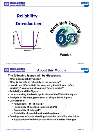
/3710 BB W4 Reliability 05, D. Szemkus/H. Winkler
Reliability
Introduction
Week 4
Failurerate--->
Time--->
Page 2/3710 BB W4 Reliability 05, D. Szemkus/H. Winkler
The following issues will be discussed:
• What does reliability mean?
• What is the role of reliability in the company?
• How do we differentiate between early life failures „infant
mortality“, random and wear out failure modes?
• Reliability and Six Sigma
• Understanding the basic application of the Weibull analysis
• Analysis of life time, generation of simple Weibull plots
• Calculation of
• Failure rate – MTTF / MTBF
• Probability of success (surviving) (Ps)
• Probability of failure (Pf)
• Reliability of parallel und serial systems
• Development of understanding about the reliability allocation
• Application of reliability allocations in system - designs
About this Module…

What is Reliability ?
Reliability is the probability, that a product or a
system…
• …does not work as intended
• …within specified limits
• …under determined conditions
• …over a predetermined time frame
What is Classic Reliability ?
43210
0.9
0.8
0.7
0.6
0.5
0.4
0.3
0.2
0.1
0.0
C1
C2
R(t)
t
Reliability in a Weibull Distribution
• The probability, that a part or system fails…
• After a specified time
• In a defined environment
We say, R(T0) = Pr(T>T0)
What can be the causes for
an early failure or
breakdown?

Why is Reliability so Important ?
• Customers expect reliability
• It saves the customer money
• A deciding factor to
• …hold customers
• …win back lost customers
• …win new customers
• It save us money
• Costs to correct one single defect:
– €34 during development
– €177 before procurement
– €368 before production
– €17,000 before shipment
– €690,000 at the customer
• The cost to correct a satellite are much higher…
Cost data from 1991 EuroPACE Quality Forum, Horoshi Hamada, President of Ricoh
The consideration and development of reliability has to be performed
early in the product development
What are the Costs of a Reliability Problem ?

Reliability – 3 Phases
Product failure can occur in three phases
•The first phase we call it the „infant
mortality“ period, characterized by
a high failure rate at the beginning,
its decreasing over time.
•The second phase is characterized
by random failures. Failure
possibilities are independent of
time.
•The third phase we call it wear out
period, characterized by an
increasing failure rate over time.
First Phase
“infant mortality”
Third Phase
wear out
Failurerate
Time--->
Second Phase
- Design Life Time -
Reliability Consideration – Phases 1 & 3
For the reliability calculation both areas have to be included:
1. Infant mortality → Corrective actions, usually a design change.
Characteristically is the tendency to a decreasing failure rate after the field
implementation (not predictable defects)
2. Wear out → Corrective actions are normally parts or components
replacement (predictable defect)
failurerate
time--->
Requirement
Minimal design life (hours / years)
random
Infant mortality
wear out
AcceptableNot acceptable

System Planning & Requirement Definition
• Serial reliability:
The reliability of one single component influences the reliability of the
system if serial connected.
The failure of one component results in a failure of the complete
system.
Basics for reliability of components
R4
R1
R2
R3
V+
V-
V out
-
+
R1 R2 R3
R4 X1
Example: Electrical circuit Block diagram for reliability
• Parallel reliability:
The system is functioning also of a failure of some components.
Computer
1
Computer
2
Computer
3
Computer 1, 2, and 3
have the same function,
parallel connected.
Only 1 computer of 3 is
needed for a proper function.
Example:
Basics for reliability of components

Probability of success
• Reliability → Probability of success (Ps):
Definition: The probability of success or survival (Ps) is the probability
that a component or system is in operation up to a determined point of
time.
Ps = 1 for a perfect reliable system
Ps = 0 for a total unreliability System
• Unreliability → Probability of failure (Pf):
Definition: The probability of failures (Pf) is the probability that a
component or system fails or does not work anymore before a
determined point of time.
Ps + Pf = 1
for all systems
• Exponential distribution function
e = natural Logarithm (2,718281828)
λ = failure rate
t = time, mostly expressed in hours
• MTBF: Mean Time Between Failures
Average failure time or reciprocal
value of the failure rate
t
ePs λ−
=
MTBF
1
=λ

h
Failure
0002.0
Failure
h
5000
11
===
MTBF
λ
4966.0)3500)(0002.0(
=== −λ−
eePs t
Example 1:
The MTBF of a systems is 5000 h. What is the probability,
that the system is still in operation at 3500 h?
Serial system
System components are serial connected, so that the failure of one
component result in a failure of the whole system.
component
2
component
3
component
1
Ps(System) = Ps(1) x Ps(2) x Ps(3) x …

Example 2: Simple serial system
Each of the 3 components (system) has a MTBF of 5000 h. What is
the probability, if serial connected, that the system is still in
operation after 1000 h?
component 2
MTBF = 5000 h
component 3
MTBF = 5000 h
component 1
MTBF = 5000 h
h
Failure
0002.0=λ
8187.0)1000)(0002.0(
)3()2()1(
==== −
ePsPsPs
549.0)3()2()1()(
=××= PsPsPsPs System
Example 2: alternative solution
Because the 3 components are build in series, we can sum the
individual failure rates before the calculation of the value Ps(System)
h
Failure
system 0006.0321 =++= λλλλ
h
Failure
0002.0=λ
549.0)1000)(0006.0(
)(
== −
ePs System

Simple parallel system
System components are connected „or“ that a failure of one
component does not result in a failure of the complete system .
component
2
component
1
Ps(System) = 1 – (Pf(1) x Pf(2))
Example 3:
Two components are parallel connected, each has a MTBF of 5000
h. What is the probability that the complete system is still in
operation after 3500 h?
component 2
MTBF = 5000 h
component 1
MTBF = 5000 h
0002.0
1
==λ
MTBF
4966.0)3500)(0002.0(
21 === −
ePsPs
7466.0)4966.01)(4966.01(1*1 21 =−−−=−= PfPfPssystem

Serial - parallel systems
The reliability of more complex systems can be calculated with a so
called serial and parallel combination technique.
A/B/C D/E F A/B/C/D/E/FB
A
C
E
D
F
1
2
3
Example 4: The complex Model in Step 1 can be reduced in accordance to
step 2 and than again in accordance to step 3
Additional analysis techniques for systems
B
A
C
D…
AB
A
C
B
A
C
D
B
A
D
C
E
X components, Y required Dependent elements
Time dependent failure
rates (simple)
Time dependent failure
rates (complex)
Reparable Systems
Method:
Binomial distribution
Method:
Markov Modeling
Method:
•Calculation of
probability distributions
•Mont Carlo Simulation
Method:
Monte Carlo Simulation
Method:
Markov Modeling
Monte Carlo Simulation

RELIABILITY PREDICTION
• Prediction is based on a model combining failure rates of
the individual components and/or subsystems to provide
an overall picture of product/equipment reliability
• Most models are built on an exponential (constant) failure
rate that is additive
• The process of modeling requires understanding of
component/subsystem reliability, use, and stress levels
Conclusion
• Provides a ball park estimate of failure rates and serves as a
comparison between products
• Provides guidance for the selection of components - It is highly
recommended that you thoroughly understand the reliability of
high failure rate parts and subsystems
• Highlights the stress levels on each part - It is highly
recommended that a thorough stress level review be done for
each component, joint, fastener, connector, etc.
Example 5:
A serial system contains 3 components. What should be the
required MTBF for component 1, that the overall system achieves a
Ps = 0,85 at 1000 operating hours?
component 2
MTBF = 20.000 h
Ps = 0,951
component 3
MTBF = 12.500 h
Ps = 0,923
component 1
MTBF = ?

Failure Mechanism
Over stressing:
• Mechanic
•Disruption
•Overload
•Thermal
•Electrical
•Electrostatic charging
•Chemical
•Contamination
•Others, incl. radiation etc.
Wear out:
• Mechanic
•Endurance stress
•Wear
•Thermal
•Electrical
•Chemical
•Corrosion
•Polymerization
•Diffusion
•Others
Definition of Ps…
Ps = Probability of success
Example:
The marketing department likes to operate some LEDs
with 13 V (designed for 6,3 V) in order to get a brighter
bill board for an exhibition.
Question, what life time can we expect life at a voltage of
13 V until 10% of the LEDs failed?

The Weibull - Analysis
Weibull- Basics
• Each Weibull – Plot presents a failure of the same
failure type (failure mode / phase)
• To define the failure time precise three requirements
have to be fulfilled:
• The failure time has to be measured clearly
• A consistent metric for the expired time
• The meaning of the failure who is causing the break
down must be clearly defined
Stat
>Reliability/Survival
>Distribution Analysis
(Right Censoring)
>Distribution ID Plot
Stat
(Right Censoring)
>Distribution ID Plot
Simple and short example:
The time to failure is measured for 2 products. 18 samples of product A shows a
variation between 10 – 66 hours.
Lets generate with these numbers some distribution plots.
1. Check if Weibull distribution fits.
RELIABILITY1.mtw

The Anderson-Darling statistic indicates
that a smaller value has a better fit of the
data.
The default setting result in Pearson
correlation coefficients. Here the best fit
is 1 or –1.
For these data the Weibull distribution
fits. Normal and Lognormal can be taken
as well.
T T F A
Percent
10010
90
50
10
1
T T F A
Percent
10010
99
90
50
10
1
T T F A
Percent
100,010,01,00,1
90
50
10
1
T T F A
Percent
7550250
99
90
50
10
1
C orrelation C oefficient
Weibull
0,986
Lognormal
0,974
Exponential
*
Normal
0,981
Probability Plot for TTF A
LSXY Estimates-Complete Data
Weibull Lognormal
Exponential Normal
T T F A
Percent
10010
90
50
10
1
T T F A
Percent
10010
99
90
50
10
1
T T F A
Percent
100,010,01,00,1
90
50
10
1
T T F A
Percent
7550250
99
90
50
10
1
A nderson-Darling (adj)
Weibull
0,983
Lognormal
1,109
Exponential
2,736
Normal
1,040
ML Estimates-Complete Data
Weibull Lognormal
Exponential Normal
Option: Maximum Likelihood
2. Set up the graphic
You can define the min & max value
for the x- coordinate for better
visibility.
Stat
(Right Censoring)
>Parametric Distribution
analysis
Stat
(Right Censoring)
analysis

TTF A
Percent
100101
99
90
80
70
60
50
40
30
20
10
5
3
2
1
Table of Statistics
Median 34,9921
IQ R 26,3116
Failure 18
C ensor 0
A D* 0,898
Shape
C orrelation 0,986
2,04782
Scale 41,8503
Mean 37,0755
StDev 18,9726
Complete Data - LSXY Estimates
Weibull - 95% CI
Beta
Eta
The values Beta and Eta – the meaning
• The Beta (β) value indicates the slope of the calculated
straight line which is linked to the failure mechanism.
Within the Minitab graphic you find the Beta value
under „Shape“.
• The Eta (η) value is also calculated by Minitab (as
Scale) and presents the characteristic design life. That
is the intersection on the line corresponding 63,2 %
with the calculated straight line. With other words, 63,2
% of the parts will fail at that characteristic design life!
At β = 1 means η the characteristic design life
MTTF (Mean Time to Failure) or MTBF (Mean Time Between Failure)

The meaning of the Beta (β) value / the slope
• What is the size of the Beta value in our example and what is the
conclusion in respect the failure cause?
• A β < 1 indicates to a “infant mortality” early failure rate
• Insufficient „burn-in“ or „stress screening“
• Production problems, wrong assembly, quality control
• Overhaul problems
• A β ≈ 1 indicates to a random failure
• Maintenance failure, human error
• Defects due to natural influence, „FOD“
• Combination of 3 or more failure reasons (different β)
• Intervals between failures
• A 1 < β < 4 indicates to a failure due to early wear out
• Low Cycle Fatigue
• Mostly bearing defects
• Corrosion, Erosion
• A β > 4 indicates to an old age (sudden) wear out
• Stress corrosion
• Material conditions
• Material break out, similar to ceramic
The meaning of the Beta (β) value / the slope

What do we understand of „B“ design life?
• „B“ design life (e.g. B10, B50, etc.) refers to the time at
10% or 50%, etc. of the parts (components) did fail. The
„TTF A“ design life can be read off on the x- axis of our
plot.
• List the numbers for „TTF A“ from our example:
• B1
• B10
• B50
• If the warranty time is 20 hours, how much % of the
parts do we expect to fail up to this point of time?
Values from the Session
Window in Minitab:
B1 = 4,4
B10 = 13,9
B50 = 35,0
B90 = 62,9
After 20 hours about 20%
have failed
Standard 95,0% Normal CI
Percent Percentile Error Lower Upper
1 4,42708 2,32142 1,58407 12,3726
2 6,22574 2,82416 2,55896 15,1467
3 7,60788 3,13729 3,39040 17,0717
4 8,77741 3,36320 4,14205 18,6002
5 9,81277 3,53796 4,84054 19,8925
6 10,7540 3,67882 5,50025 21,0260
7 11,6247 3,79550 6,13003 22,0446
8 12,4403 3,89402 6,73587 22,9758
9 13,2115 3,97840 7,32200 23,8384
10 13,9460 4,05147 7,89162 24,6453
20 20,1186 4,44800 13,0439 31,0305
30 25,2967 4,58931 17,7271 36,0984
40 30,1468 4,66300 22,2629 40,8227
50 34,9921 4,75897 26,8044 45,6809
60 40,1013 4,96171 31,4659 51,1066
70 45,8211 5,38916 36,3876 57,7003
80 52,7986 6,25718 41,8549 66,6038
90 62,8893 8,16007 48,7676 81,1004
91 64,2785 8,47424 49,6417 83,2310
92 65,7951 8,82996 50,5777 85,5910
93 67,4713 9,23788 51,5913 88,2393
94 69,3537 9,71355 52,7050 91,2614
95 71,5132 10,2809 53,9530 94,7888
96 74,0666 10,9798 55,3909 99,0391
97 77,2284 11,8845 57,1198 104,416
98 81,4671 13,1599 59,3583 111,811
99 88,2220 15,3251 62,7645 124,005

Lets compare the two product designs. Now we want to see if the modification
results in a significant difference for time to failure.
Analyze it with the support of Weibull Plots
Stat
(Right Censoring)
analysis
TTF
Percent
100101
99
90
80
70
60
50
40
30
20
10
5
3
2
1
Table of Statistics
18 0
4,51847 101,793 0,982 26 0
Shape Scale C orr F C
2,04782 41,850 0,986
Product
TTF A
TTF B
Probability Plot for TTF
Complete Data - LSXY Estimates
Weibull - 95% CI
Beta
Eta
What do you conclude from the analysis?

Definition of Ps…
Ps = Probability of success
Example:
The marketing department likes to operate some LEDs
with 13 V (designed for 6,3 V) in order to get a brighter
bill board for an exhibition.
Question, what life time can we expect life at a voltage of
13 V until 10% of the LEDs failed?
Failure time of the LEDs: 867, 802, 882 und 935 sec.
What failure type results from the Beta value?

Javier Garcia - Verdugo Sanchez - Six Sigma Training - W4 Reliability

Recommended

Recommended

More Related Content

What's hot

What's hot (20)

Viewers also liked

Viewers also liked (13)

Similar to Javier Garcia - Verdugo Sanchez - Six Sigma Training - W4 Reliability

Similar to Javier Garcia - Verdugo Sanchez - Six Sigma Training - W4 Reliability (20)

More from J. García - Verdugo

More from J. García - Verdugo (20)

Recently uploaded

Recently uploaded (20)

Javier Garcia - Verdugo Sanchez - Six Sigma Training - W4 Reliability