Testing of hypotheses

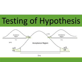
/2
CR
/2
CR
1-
Acceptance Region
Testing of Hypothesis

(CR)
1-
Acceptance
Region
(RTT)
 (CR)
1-
Acceptance
Region

Testing of Hypotheses
Hypothesis : Any assumption regarding the population
parameters is called hypothesis. Or to predict the results of
an event before experiment is called hypothesis. It is of
following types
1. Statistical Hypothesis
a. Null hypothesis
b. Alternative hypothesis
2. Simple and composite hypothesis
3. Research hypothesis

Null Hypothesis
The basic assumption regarding population parameters
which can be tested is called null hypothesis.
In the other word any statement that may difference
between observed sample statistics and specified
population parameter is due to a sampling error is called
null hypothesis.
Therefore the null hypothesis means hypothesis of no
different and it is denoted by H0

Alternative Hypothesis
When the null hypothesis is rejected than the
assumption taken as true is called alternative
hypothesis and it is denoted by H1
Simple and Composite Hypothesis
If all the unknown parameter of the distribution
are specified by the hypothesis then it is called
simple hypothesis. If at least one parameter
remain unspecified then it called composite
hypothesis.

For Example
The hypothesis population is normal with mean 25 and Standard Deviation 5 is
a simple hypothesis where as the hypothesis population is normal with mean
25 is a composite hypothesis
Research Hypothesis
It is an declarative expected relationship or the
difference between two variable in other words
what relationship the research except to verity
through the collection and analysis of data and it
gives the tentative answer to the research question.
For Ex. –The Train teacher leads better performance
through untrained teacher.

Testing of Hypothesis
Testing of hypothesis is nothing but to divide the
sample space into two parts acceptance region and
critical region.
Now to specify the critical region with in the sample
space is called testing of hypothesis. When ever the
decision are taken in the basis of sampling, the
following four possibilities will be there.

1. Null Hypothesis (H0) : Was true and the sample point lies in
acceptance region, thus a true hypothesis is accepted and it is a
correct decision.
2. Null Hypothesis (H0) : Was true but the sample points lies in
critical region, thus a true hypothesis is rejected and it is a wrong
decision called type-I error. It’s probability is denoted by α .
α = P[Type-I error]
= P[rejecting H0, while H0 is true]
= P[Point lies in CR under H0]
= area of CR under H0

3. Null Hypothesis (H0) : Was false, but the
sample points lies in acceptance region. Thus
a false hypothesis is accepted, it is a wrong
decision called type-II error and its probability
is denoted by 
 = P[type-II error]
= P[Accepting H0, while H0 is false]
= P[Point lies in AR under H1]
= Area of AR under H1

4. Null Hypothesis (H0) : Was false and the
sample point lies in CR, thus a wrong hypothesis
is rejected it is a correct decision and its
probability is denoted by power.
Power = P[Rejecting H0, While H0 is false]
= P[Point lies in CR under H1]
= Area of CR under H1
Power = 1- 

Level of Significance
The maximum size of type-I error that we are
prepared to take risk is called the level of
significance. In other word the probability of
rejecting a true hypothesis is called level of
significance and it is denoted by .
Hypothesis generally are tested at 1% or 5%
level of significance, but the most commonly
used level of significance in practice is 5%.
If We adopted =5% LS it shows that in 5 true
samples out of 100 are likely to be reject a
correct hypothesis.

Critical region and acceptance region
The region where true null hypothesis is rejected is called Critical Region.
But The region for accepting true null hypothesis is called acceptance
region.
/2
CR
/2
CR
1-
Acceptance Region

One tailed and two tailed test
One tailed and two tailed test, depends upon the situation of critical
region on the tails of the standard normal curve which is symmetrical
about mean and the total area covered is unity. In other words, if an
alternative hypothesis leads to two alternations to the null hypothesis, it
is said to be a two tailed test as the critical region is found to be situated
on both the tails.
OR
One Tailed test : Any test where the critical region consists only of one
tail of the sampling distribution of the test is called one tailed test
For Example :
Null Hypothesis (H0) : =0
Alternative Hypothesis (H1) :>0 (Right tailed test)
OR
Alternative Hypothesis (H1) :<0 (Left tailed test)

Two tailed test
Any test where the Critical Region consists only of two tail of the
sampling distribution of the test statistics called two tailed test
For Example :
Alternative Hypothesis (H1) :0 (Two tailed test)
 (CR)
1-
Acceptance Region
(RTT)
(LTT)
(TTT)
 (CR)
1-
Acceptance Region
/2
CR
1-
Acceptance Region
/2
CR

Identification of One Tailed and
Two Tailed Test
There is no any hard and fast rule to identify the one tailed and two tailed test of
hypothesis. Generally, if direction of differences is not given in the statement of
hypothesis, then we use two tailed test. Similarly if the direction of difference like
at least, at most, increase, decrease, majority, minority, larger, taller, high, low,
superior, inferior, improved, more than, less than etc is included in the statement
of hypothesis, then we use one tailed test.

Steps of Testing of Hypothesis
1. State the null and alternative hypothesis
2. Choose the level of significance at size 
3. Determine the critical region
4. Use test statistic
5. Making decision or conclusion

A test statistic is a sample statistic computed from sample
data. The value of the test statistic is used in determining
whether or not we may reject the null hypothesis.
The decision rule of a statistical hypothesis test is a rule that
specifies the conditions under which the null hypothesis may
be rejected.
7-2 The Concepts of
Hypothesis Testing
Consider H0: = 100. We may have a decision rule that says: “Reject H0 if the sample
mean is less than 95 or more than 105.”
In a courtroom we may say: “The accused is innocent until proven guilty beyond a
reasonable doubt.”

• There are two possible states of nature:
H0 is true
H0 is false
• There are two possible decisions:
Fail to reject H0 as true
Reject H0 as false
Decision Making

• A decision may be correct in two ways:
Fail to reject a true H0
Reject a false H0
• A decision may be incorrect in two ways:
Type I Error: Reject a true H0
• The Probability of a Type I error is denoted
by .
Type II Error: Fail to reject a false H0
• The Probability of a Type II error is denoted
by .
Decision Making

A decision may be incorrect in two ways:
Type I Error: Reject a true H0
◦ The Probability of a Type I error is denoted by .
◦ is called the level of significance of the test
Type II Error: Accept a false H0
◦ The Probability of a Type II error is denoted by .
◦ 1 - is called the power of the test.
and are conditional probabilities:


Errors in Hypothesis Testing


= P(Reject H H is true)
= P(Accept H H is false)
0 0
0 0

A contingency table illustrates the possible outcomes
of a statistical hypothesis test.
Type I and Type II Errors

The p-value is the probability of obtaining a value of the test statistic as extreme as,
or more extreme than, the actual value obtained, when the null hypothesis is true.
The p-value is the smallest level of significance, , at which the null hypothesis
may be rejected using the obtained value of the test statistic.
Policy: When the p-value is less than a , reject H0.
The p-Value
NOTE: More detailed discussions about the p-value will be given later in the
chapter when examples on hypothesis tests are presented.

The power of a statistical hypothesis test is the
probability of rejecting the null hypothesis when the
null hypothesis is false.
Power = (1 - )
The Power of a Test

The probability of a type II error, and the power of a test, depends on the actual value
of the unknown population parameter. The relationship between the population mean
and the power of the test is called the power function.
7069686766656463626160
1.0
0.9
0.8
0.7
0.6
0.5
0.4
0.3
0.2
0.1
0.0
Power of a One-Tailed Test: =60, =0.05
Power
Value of m b Power = (1 - b)
61 0.8739 0.1261
62 0.7405 0.2695
63 0.5577 0.4423
64 0.3613 0.6387
65 0.1963 0.8037
66 0.0877 0.9123
67 0.0318 0.9682
68 0.0092 0.9908
69 0.0021 0.9972
The Power Function

The power depends on the distance between the value of
the parameter under the null hypothesis and the true value
of the parameter in question: the greater this distance, the
greater the power.
The power depends on the population standard deviation:
the smaller the population standard deviation, the greater
the power.
The power depends on the sample size used: the larger the
sample, the greater the power.
The power depends on the level of significance of the test:
the smaller the level of significance,, the smaller the
power.
Factors Affecting the Power
Function

A company that delivers packages within a large metropolitan area claims that it takes
an average of 28 minutes for a package to be delivered from your door to the
destination. Suppose that you want to carry out a hypothesis test of this claim.
We can be 95% sure that the average time for
all packages is between 30.52 and 32.48
minutes.
Since the asserted value, 28 minutes, is not
in this 95% confidence interval, we may
reasonably reject the null hypothesis.
Set the null and alternative hypotheses:
H0: = 28
H1: 28
Collect sample data:
n = 100
x = 31.5
s = 5
Construct a 95% confidence interval for
the average delivery times of all packages:
 
x z
s
n
  
  
.
. .
. . . , .
025
315 196
5
100
315 98 3052 32 48
Example

The tails of a statistical test are determined by the need for an action. If action
is to be taken if a parameter is greater than some value a, then the alternative
hypothesis is that the parameter is greater than a, and the test is a right-tailed
test. H0: 50
H1: 50
If action is to be taken if a parameter is less than some value a, then the
alternative hypothesis is that the parameter is less than a, and the test is a left-
tailed test. H0: 50
H1: 50
If action is to be taken if a parameter is either greater than or less than some
value a, then the alternative hypothesis is that the parameter is not equal to a,
and the test is a two-tailed test. H0: 50
H1: 50
7-3 1-Tailed and 2-Tailed Tests

We will see the three different types of hypothesis tests, namely
Tests of hypotheses about population means
Tests of hypotheses about population proportions
Tests of hypotheses about population proportions.
7-4 The Hypothesis Tests

• Cases in which the test statistic is Z
s is known and the population is normal.
s is known and the sample size is at least 30. (The population need not be normal)
Testing Population Means








n
x
z
isZgcalculatinforformulaThe


:

• Cases in which the test statistic is t
s is unknown but the sample standard deviation is known and the population is
normal.
Testing Population Means








n
s
x
t
istgcalculatinforformulaThe

:

The rejection region of a statistical hypothesis test
is the range of numbers that will lead us to reject the
null hypothesis in case the test statistic falls within
this range. The rejection region, also called the
critical region, is defined by the critical points.
The rejection region is defined so that, before the
sampling takes place, our test statistic will have a
probability of falling within the rejection region if
the null hypothesis is true.
Rejection Region

The non rejection region is the range of values
(also determined by the critical points) that will lead
us not to reject the null hypothesis if the test statistic
should fall within this region. The non rejection
region is designed so that, before the sampling takes
place, our test statistic will have a probability 1- of
falling within the non rejection region if the null
hypothesis is true
In a two-tailed test, the rejection region consists of the
values in both tails of the sampling distribution.
Nonrejection Region

= 28 32.4830.52 x = 31.5
Population
mean under H0
95% confidence
interval around
observed sample mean
It seems reasonable to reject the null hypothesis, H0: = 28, since the
hypothesized value lies outside the 95% confidence interval. If we’re 95% sure
that the population mean is between 30.52 and 32.58 minutes, it’s very unlikely
that the population mean is actually be 28 minutes.
Note that the population mean may be 28 (the null hypothesis might be true), but
then the observed sample mean, 31.5, would be a very unlikely occurrence. There’s
still the small chance ( = .05) that we might reject the true null hypothesis.
represents the level of significance of the test.
Picturing Hypothesis Testing

If the observed sample mean falls within the nonrejection region, then you fail to
reject the null hypothesis as true. Construct a 95% nonrejection region around
the hypothesized population mean, and compare it with the 95% confidence
interval around the observed sample mean:
 
0 025
28 196
5
100
28 98 27 02 28 98
  
  
z
s
n.
.
. , , .
x 32.4830.52
95% Confidence
Interval
around the
Sample Mean
0=28 28.9827.02
95% non-
rejection region
around the
population Mean  
x z
s
n
  
  
.
. .
. . . ,
025
315 196
5
100
315 98 3052 32.48
The nonrejection region and the confidence interval are the same width, but
centered on different points. In this instance, the nonrejection region does not
include the observed sample mean, and the confidence interval does not include
the hypothesized population mean.
Nonrejection Region

T
0.8
0.7
0.6
0.5
0.4
0.3
0.2
0.1
0.0
he Hypothesized Sampling Distribution of the Mean
0=28 28.9827.02
.025 .025
.95
If the null hypothesis were true,
then the sampling distribution of
the mean would look something
like this:
We will find 95% of the
sampling distribution between
the critical points 27.02 and 28.98,
and 2.5% below 27.02 and 2.5% above 28.98 (a two-tailed test). The 95% interval
around the hypothesized mean defines the nonrejection region, with the remaining 5%
in two rejection regions.
Picturing the Nonrejection and
Rejection Regions

Nonrejection
Region
Lower Rejection
Region
Upper Rejection
Region
0.8
0.7
0.6
0.5
0.4
0.3
0.2
0.1
0.0
The Hypothesized Sampling Distributionof the Mean
0=28 28.9827.02
.025 .025
.95
x
Construct a (1- ) nonrejection region around the hypothesized
population mean.
Do not reject H0 if the sample mean falls within the nonrejection region
(between the critical points).
Reject H0 if the sample mean falls outside the nonrejection region.
The Decision Rule

An automatic bottling machine fills cola into two liter (2000 cc) bottles. A consumer advocate wants to test the null
hypothesis that the average amount filled by the machine into a bottle is at least 2000 cc. A random sample of 40
bottles coming out of the machine was selected and the exact content of the selected bottles are recorded. The
sample mean was 1999.6 cc. The population standard deviation is known from past experience to be 1.30 cc.
Test the null hypothesis at the 5% significance level.
H0: 2000
H1: 2000
n = 40
For = 0.05, the critical value
of z is -1.645
The test statistic is:
Do not reject H0 if: [z -1.645]
Reject H0 if: z ]
z
x
s
n

 0
0
HReject1.95=
=0
1.3=
1999.6=x
40=n
40
1.3
2000-1999.6



n
x
z



Example 7-5

An automatic bottling machine fills cola into two liter (2000 cc) bottles. A consumer advocate wants to test the null
hypothesis that the average amount filled by the machine into a bottle is at least 2000 cc. A random sample of 40
bottles coming out of the machine was selected and the exact content of the selected bottles are recorded. The
sample mean was 1999.6 cc. The population standard deviation is known from past experience to be 1.30 cc.
Test the null hypothesis at the 5% significance level.
H0: 2000
H1: 2000
n = 40
of z is -1.645
Do not reject H0 if: [p-value 0.05]
Reject H0 if: p-value 0.0 ]
z
x
s
n

 0
0.050.0256since
0
HReject0.0256
0.4744-0.5000
1.95)-P(Zvalue-
1.95=
=0
40
1.3
2000-1999.6






p
n
x
z


Example 7-5: p-value
approach

Example 7-5: Using the
Template
Use when s is
known
Use when s is
unknown

Example 7-6: Using the Template
with Sample Data
Use when s is
known
Use when s is
unknown

• Cases in which the binomial distribution can be used
The binomial distribution can be used whenever we are able to calculate the necessary
binomial probabilities. This means that for calculations using tables, the sample size n
and the population proportion p should have been tabulated.
Note: For calculations using spreadsheet templates, sample sizes up to 500 are
feasible.
Testing Population Proportions

• Cases in which the normal approximation is to be used
If the sample size n is too large (n > 500) to calculate binomial probabilities then the
normal approximation can be used.and the population proportion p should have been
tabulated.
Testing Population Proportions

A coin is to tested for fairness. It is tossed 25 times and only 8 Heads are observed. Test
if the coin is fair at an a of 5% (significance level).
Example 7-7: p-value
approach
Let p denote the probability of a Head
H0: p = 0.5
H1: p 0.5
Because this is a 2-tailed test, the p-value = 2*P(X 8)
From the binomial tables, with n = 25, p = 0.5, this value
2*0.054 = 0.108.s
Since 0.108 > = 0.05, then
do not reject H0

with the Binomial Distribution

with the Normal Distribution

• For testing hypotheses about population variances, the test statistic (chi-square) is:
where is the claimed value of the population variance in the null hypothesis. The
degrees of freedom for this chi-square random variable is (n – 1).
Note: Since the chi-square table only provides the critical values, it cannot
be used to calculate exact p-values. As in the case of the t-tables, only a
range of possible values can be inferred.
Testing Population Variances
 
2
0
2
2 1


sn 

2
0


A manufacturer of golf balls claims that they control the weights of the golf balls
accurately so that the variance of the weights is not more than 1 mg2. A random sample
of 31 golf balls yields a sample variance of 1.62 mg2. Is that sufficient evidence to reject
the claim at an a of 5%?
Example 7-8
Let s2 denote the population variance. Then
H0: s2 < 1
H1: s2 > 1
In the template (see next slide), enter 31 for the sample size
and 1.62 for the sample variance. Enter the hypothesized value
of 1 in cell D11. The p-value of 0.0173 appears in cell E13. Since
This value is less than the a of 5%, we reject the null hypothesis.

As part of a survey to determine the extent of required in-cabin storage capacity, a
researcher needs to test the null hypothesis that the average weight of carry-on baggage
per person is 0 = 12 pounds, versus the alternative hypothesis that the average weight
is not 12 pounds. The analyst wants to test the null hypothesis at = 0.05.
H0: = 12
H1: 12
For = 0.05, critical values of z are ±1.96
Do not reject H0 if: [-1.96 z 1.96]
Reject H0 if: [z <-1.96] or z 1.96]
z
x
s
n

 0
Lower Rejection
Region
Upper Rejection
Region
0.8
0.7
0.6
0.5
0.4
0.3
0.2
0.1
0.0
.025 .025
.95
Nonrejection
Region
z1.96-1.96
The Standard Normal Distribution
Additional Examples (a)

n = 144
x = 14.6
s = 7.8
=
14.6-12
7.8
144
=
2.6
0.65
z
x
s
n



0
4
Since the test statistic falls in the upper rejection region, H0 is rejected, and we may
conclude that the average amount of carry-on baggage is more than 12 pounds.
Lower Rejection
Region
Upper Rejection
Region
0.8
0.7
0.6
0.5
0.4
0.3
0.2
0.1
0.0
.025 .025
.95
Nonrejection
Region
z1.96-1.96
Additional Examples (a):
Solution

An insurance company believes that, over the last few years, the average liability
insurance per board seat in companies defined as “small companies” has been $2000.
Using = 0.01, test this hypothesis using Growth Resources, Inc. survey data.
H0: = 2000
H1: 2000
Reject H0 if: [z <-2.576] or z 2.576]
z
x
s
n

 0
n = 100
x = 2700
s = 947
=
2700 - 2000
947
100
=
700
94.7
Reject H
0
z
x
s
n


 
0
7 39.
Additional Examples (b)

Since the test statistic falls in the upper
rejection region, H0 is rejected, and we
may conclude that the average insurance
liability per board seat in “small
companies” is more than $2000.
Lower Rejection
Region
Upper Rejection
Region
0.8
0.7
0.6
0.5
0.4
0.3
0.2
0.1
0.0
.005 .005
.99
Nonrejection
Region
z2.576-2.576
Additional Examples (b) :
Continued

The average time it takes a computer to perform a certain task is believed to be 3.24
seconds. It was decided to test the statistical hypothesis that the average performance
time of the task using the new algorithm is the same, against the alternative that the
average performance time is no longer the same, at the 0.05 level of significance.
H0: = 3.24
H1: 3.24
Reject H0 if: [z < -1.96] or z 1.96]
z
x
s
n

 0
n = 200
x = 3.48
s = 2.8
=
200
= Do not reject H
0
3.48- 3.24
2.8
0.24
0.20
z
x
s
n


 
0
1 21.
Additional Examples (c)

Since the test statistic falls in the
nonrejection region, H0 is not rejected,
and we may conclude that the average
performance time has not changed from
3.24 seconds.
Lower Rejection
Region
Upper Rejection
Region
0.8
0.7
0.6
0.5
0.4
0.3
0.2
0.1
0.0
.025 .025
.95
Nonrejection
Region
z1.96-1.96
Additional Examples (c) :
Continued

According to the Japanese National Land Agency, average land prices in central Tokyo
soared 49% in the first six months of 1995. An international real estate investment
company wants to test this claim against the alternative that the average price did not rise
by 49%, at a 0.01 level of significance.
H0: = 49
H1: 49
n = 18
For = 0.01 and (18-1) = 17 df ,
critical values of t are ±2.898
Do not reject H0 if: [-2.898 t 2.898]
Reject H0 if: [t < -2.898] or t 2.898]
0
HReject33.3=
=0
14=s
38=x
18=n
3.3
11-
18
14
49-38



n
s
x
t

t
x
s
n

 0
Additional Examples (d)

may conclude that the average price has
not risen by 49%. Since the test statistic
is in the lower rejection region, we may
conclude that the average price has risen
by less than 49%.
Lower Rejection
Region
Upper Rejection
Region
0.8
0.7
0.6
0.5
0.4
0.3
0.2
0.1
0.0
.005 .005
.99
Nonrejection
Region
t2.898-2.898
The t Distribution
Additional Examples (d) :
Continued

Canon, Inc,. has introduced a copying machine that features two-color copying capability
in a compact system copier. The average speed of the standard compact system copier is
27 copies per minute. Suppose the company wants to test whether the new copier has the
same average speed as its standard compact copier. Conduct a test at an = 0.05 level
of significance.
H0: = 27
H1: 27
n = 24
For = 0.05 and (24-1) = 23 df ,
critical values of t are ±2.069
Do not reject H0 if: [-2.069 t 2.069]
Reject H0 if: [t < -2.069] or t 2.069]
0
HrejectnotDo59.1=
=0
7.4=s
24.6=x
24=n
1.51
2.4-
24
7.4
27-24.6



n
s
x
t

0
n
s
x
t


Additional Examples (e)

and we may not conclude that the
average speed is different from 27 copies
per minute.
Lower Rejection
Region
Upper Rejection
Region
0.8
0.7
0.6
0.5
0.4
0.3
0.2
0.1
0.0
.025 .025
.95
Nonrejection
Region
t2.069-2.069
The t Distribution
Additional Examples (e) :
Continued

While the null hypothesis is maintained to be true throughout a hypothesis
test, until sample data lead to a rejection, the aim of a hypothesis test is often
to disprove the null hypothesis in favor of the alternative hypothesis. This is
because we can determine and regulate , the probability of a Type I error,
making it as small as we desire, such as 0.01 or 0.05. Thus, when we reject a
null hypothesis, we have a high level of confidence in our decision, since we
know there is a small probability that we have made an error.
A given sample mean will not lead to a rejection of a null hypothesis unless it
lies in outside the nonrejection region of the test. That is, the nonrejection
region includes all sample means that are not significantly different, in a
statistical sense, from the hypothesized mean. The rejection regions, in turn,
define the values of sample means that are significantly different, in a
statistical sense, from the hypothesized mean.
Statistical Significance

An investment analyst for Goldman Sachs and Company wanted to test the hypothesis
made by British securities experts that 70% of all foreign investors in the British market
were American. The analyst gathered a random sample of 210 accounts of foreign
investors in London and found that 130 were owned by U.S. citizens. At the  = 0.05
level of significance, is there evidence to reject the claim of the British securities
experts?
H0: p = 0.70
H1: p  0.70
n = 210
For  = 0.05 critical values of z are ±1.96
Do not reject H0 if: [-1.96  z  1.96]
Reject H0 if: [z < -1.96] or z  1.96]
n = 210
p =
130
210
=
p - p
0
p
0
=
= Reject H
0
0.619 -0.70
(0.70)(0.30)
-0.081
0.0316
 .

.

  
0 619
0
2 5614
210
z
q
n
z
p p
p q
n

 0
0 0
Additional Examples (f)

The EPA sets limits on the concentrations of pollutants emitted by various industries. Suppose that the
upper allowable limit on the emission of vinyl chloride is set at an average of 55 ppm within a range of two
miles around the plant emitting this chemical. To check compliance with this rule, the EPA collects a
random sample of 100 readings at different times and dates within the two-mile range around the plant. The
findings are that the sample average concentration is 60 ppm and the sample standard deviation is 20 ppm.
Is there evidence to conclude that the plant in question is violating the law?
H0: 55
H1: 55
n = 100
of z is 2.326
Do not reject H0 if: [z 2.326]
Reject H0 if: z 2.326]
0
HReject5.2=
=0
20=s
60=x
100=n
2
5
100
20
55-60



n
s
x
z

z
x
s
n

 0
Additional Examples (g)

may conclude that the average
concentration of vinyl chloride is more
than 55 ppm.
0.99
2.326
50-5
0.4
0.3
0.2
0.1
0.0
z
f(z)
Nonrejection
Region
Rejection
Region
Critical Point for a Right-Tailed Test
2.5
Additional Examples (g) :
Continued

A certain kind of packaged food bears the following statement on the package: “Average net weight 12 oz.”
Suppose that a consumer group has been receiving complaints from users of the product who believe that they are
getting smaller quantities than the manufacturer states on the package. The consumer group wants, therefore, to
test the hypothesis that the average net weight of the product in question is 12 oz. versus the alternative that the
packages are, on average, underfilled. A random sample of 144 packages of the food product is collected, and it is
found that the average net weight in the sample is 11.8 oz. and the sample standard deviation is 6 oz. Given these
findings, is there evidence the manufacturer is underfilling the packages?
H0: 12
H1: 12
n = 144
of z is -1.645
Do not reject H0 if: [z -1.645]
Reject H0 if: z ]
z
x
s
n

 0
n = 144
x = 11.8
s = 6
=
= Do not reject H
0
11.8-12
6
-.2
.5
z
x
s
n


  

0
0 4
144
.
Additional Examples (h)

and we may not conclude that the
manufacturer is underfilling packages on
average.
0.95
-1.645
50-5
0.4
0 .3
0 .2
0.1
0 .0
z
f(z)
Nonrejection
Region
Rejection
Region
Critical Point for a Left-Tailed Test
-0.4
Additional Examples (h) :
Continued

A floodlight is said to last an average of 65 hours. A competitor believes that the average life of the
floodlight is less than that stated by the manufacturer and sets out to prove that the manufacturer’s
claim is false. A random sample of 21 floodlight elements is chosen and shows that the sample
average is 62.5 hours and the sample standard deviation is 3. Using =0.01, determine whether
there is evidence to conclude that the manufacturer’s claim is false.
H0: 65
H1: 65
n = 21
For = 0.01 an (21-1) = 20 df, the
critical value -2.528
Do not reject H0 if: [t -2.528]
Reject H0 if: z ]
Additional Examples (i)

may conclude that the manufacturer’s
claim is false, that the average floodlight
life is less than 65 hours.
0.95

-2.528
50-5
0.4
0.3
0.2
0.1
0.0
t
f(t)
Nonrejection
Region
Rejection
Region
Critical Point for a Left-Tailed Test
-3.82
Additional Examples (i) :
Continued

“After looking at 1349 hotels nationwide, we’ve found 13 that meet our standards.” This statement by the Small Luxury Hotels
Association implies that the proportion of all hotels in the United States that meet the association’s standards is 13/1349=0.0096. The
management of a hotel that was denied acceptance to the association wanted to prove that the standards are not as stringent as claimed
and that, in fact, the proportion of all hotels in the United States that would qualify is higher than 0.0096. The management hired an
independent research agency, which visited a random sample of 600 hotels nationwide and found that 7 of them satisfied the exact
standards set by the association. Is there evidence to conclude that the population proportion of all hotels in the country satisfying the
standards set by the Small Luxury hotels Association is greater than 0.0096?
H0: p 0.0096
H1: p 0.0096
n = 600
For = 0.10 the critical value 1.282
Do not reject H0 if: [z 1.282]
Reject H0 if: z ]
Additional Examples (j)

and we may not conclude that proportion
of all hotels in the country that meet the
association’s standards is greater than
0.0096.
0.90
1.282
50-5
0 .4
0 .3
0 .2
0 .1
0 .0
z
f(z)
Nonrejection
Region
Rejection
Region
Critical Point for a Right-Tailed Test
0.519
Additional Examples (j) : Continued

The p-value is the probability of obtaining a value of the test statistic as extreme as,
or more extreme than, the actual value obtained, when the null hypothesis is true.
The p-value is the smallest level of significance, , at which the null hypothesis
may be rejected using the obtained value of the test statistic.
The p-Value Revisited
50-5
0.4
0.3
0.2
0.1
0.0
z
f(z)
Standard Normal Distribution
0.519
p-value=area to
right of the test statistic
=0.3018
Additional Example k Additional Example g
0
0
0
0
0
f(z)
50-5
.4
.3
.2
.1
.0
z
Standard Normal Distribution
2.5
p-value=area to
right of the test statistic
=0.0062

When the p-value is smaller than 0.01, the result is called very significant.
When the p-value is between 0.01 and 0.05, the result is called significant.
When the p-value is between 0.05 and 0.10, the result is considered by some as
marginally significant (and by most as not significant).
When the p-value is greater than 0.10, the result is considered not significant.
The p-Value: Rules of Thumb

In a two-tailed test, we find the p-value by doubling the area in the tail of the
distribution beyond the value of the test statistic.
p-Value: Two-Tailed Tests
50-5
0.4
0.3
0.2
0.1
0.0
z
f(z)
-0.4 0.4
p-value=double the area to
left of the test statistic
=2(0.3446)=0.6892

The further away in the tail of the distribution the test statistic falls, the smaller is the p-
value and, hence, the more convinced we are that the null hypothesis is false and should
be rejected.
In a right-tailed test, the p-value is the area to the right of the test statistic if the test
statistic is positive.
In a left-tailed test, the p-value is the area to the left of the test statistic if the test statistic
is negative.
In a two-tailed test, the p-value is twice the area to the right of a positive test statistic or
to the left of a negative test statistic.
For a given level of significance, :
Reject the null hypothesis if and only if p-value
The p-Value and Hypothesis
Testing

One can consider the following:
Sample Sizes
b versus a for various sample sizes
The Power Curve
The Operating Characteristic Curve
7-5: Pre-Test Decisions
Note: You can use the different templates that come with the text to
investigate these concepts.

Computing and Plotting
Required Sample size.
Note: Similar
analysis can
be done when
testing for a
population
proportion.

Template
Plot of b versus
a for various n.
Note: Similar
analysis can be
done when testing
for a population
proportion.

Template
The Power
Curve
Note: Similar
analysis can be
done when testing
for a population
proportion.

Template
The Operating
Characteristic Curve
for
H0:m >= 75; s =
10; n = 40; a =
10%
Note: Similar
analysis can be
done when
testing a
population
proportion.

Testing of hypotheses

Recommended

Recommended

More Related Content

What's hot

What's hot (20)

Similar to Testing of hypotheses

Similar to Testing of hypotheses (20)

More from RajThakuri

More from RajThakuri (20)

Recently uploaded

Recently uploaded (20)

Testing of hypotheses