Phylogeny in R - Bianca Santini Sheffield R Users March 2015
•Download as PPTX, PDF•
2 likes•3,195 views

This document provides an overview of using phylogenies in comparative analysis. It discusses why phylogenies are important in comparative analysis to account for shared evolutionary history between taxa. It summarizes how re-analyzing Salisbury's data on stomatal density using independent contrasts and incorporating a phylogeny changed the conclusions. The document outlines how to obtain or generate a phylogeny and load it with trait data into R. It demonstrates using the CAPER package to conduct phylogenetic generalized least squares (pgls) to analyze traits while accounting for phylogeny, including for continuous traits and factors. It discusses visualizing and exploring phylogenies in R and other programs.

Recommended
More Related Content
What's hot
What's hot (20)
Viewers also liked
Similar to Phylogeny in R - Bianca Santini Sheffield R Users March 2015
Similar to Phylogeny in R - Bianca Santini Sheffield R Users March 2015 (20)
More from Paul Richards
More from Paul Richards (11)
Recently uploaded
Recently uploaded (20)
Phylogeny in R - Bianca Santini Sheffield R Users March 2015
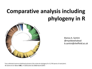
- 1. Comparative analysis including phylogeny in R AE Zanne et al. Nature 000, 1-4 (2013) doi:10.1038/nature12872 Time-calibrated maximum-likelihood estimate of the molecular phylogeny for 31,749 species of seed plants. Bianca A. Santini @myoldowlisdead b.santini@sheffield.ac.uk
- 2. What is a phylogeny? • Hypothesis that explains the evolutionary relationship among taxa* *taxa: species, or higher taxonomic levels. Also genes, or sequences node terminals/tips/leaves root A B C D Internal branch branch External branch ModifiedfromNatureScitable: http://www.nature.com/scitable/topicpage/reading-a-phylogenetic- tree-the-meaning-of-41956#
- 3. Why use phylogenies… …in comparative analysis? • Comparative analyses are used to assess the ecological significance of a particular trait • However, because there is a shared history… a) they are not statistically independent data b) the feature under study might exist because of shared ancestry
- 4. One example of data analyzed without a phylogeny • Salisbury’s data (1927, yes 88yrs ago!) • Observations – Differences in stomata density (SD) between sun(>) and shade (<) leaves • Measured stomatal density and related them to life-form, habitat type • Conclusion: SD increases with exposure SD Trees Shrubs Herbs Woody Herbs plants SD Marginal herbs Understory herbs Photo by A. Vazquez-Lobo
- 5. Re-analysis of Salisbury’s data • Independent contrasts (Felsenstein, 1985) – Introduces a phylogeny – The trait changes along the branches of the tree, should be associated to changes in the explanatory variable – no. of times the traits changes in concert with the environmental variable (agreements) vs. no. of times they do not (disagreements) – Sign test SD Trees Shrubs Herbs Woody Herbs plants SD Marginal herbs Understory herbs Kelly and Beerling, 1995 (68 yrs after)
- 6. How to get your own phylogeny ? phylomatic (uses a megatree) http://phylodiversity.net/phylomatic/ Use and trim and already published phylogeny: - Dryad: http://datadryad.org/ - Ecological Archives (from the esa) phyloGenerator (uses gen bank sequences) http://willpearse.github.io/phyloGenerator/ This is if you don’t have the sequences, or are not planning to get them.
- 7. Package CAPER : pgls() Similar approach as in Independent Contrasts, but uses a matrix of variances and covariances (tree) N.B. If interested in phylogenies and evolution analyses: geiger, adephylo, picante, phylolm, ape…
- 8. pgls: phylogenetic generalized least squares what do you need? 1. Phylogeny 2. Data – Make sure the rows in your data frame are the same as the tips of your tree i.e. your data: Juncus bufonius tree: Juncus_bufonius > my.data$underscore.name=gsub(" ","_",my.data$underscore.name) – Make sure you have one observation per species per trait: 3. Put them into a comparative.data() Species names Leaf area Seed mass Juncus_bufonius 120.2 0.24 Setaria_pumila 91.2 6.91
- 9. #1)PHYLOGENY > tree<-read.tree ("Vascular_Plants_rooted.dated.tre”) ##or read.nexus() > tree <- congeneric.merge(tree,my.data$underscore.name) ##pez package Number of species in tree before: 401 Number of species in tree now: 550 > tree Phylogenetic tree with 550 tips and 393 internal nodes. Tip labels: Gladiolus_italicus, Juncus_squarrosus, Juncus_bufonius, Bolboschoenus_maritimus, Isolepis_setacea, Cyperus_fuscus, ... Node labels: , , , , , , … Rooted; includes branch lengths. pgls() #You can always check for synonyms and replace (taxize) > my.data$underscore.name<-recode(my.data$underscore.name, "'Aegilops_geniculata' = 'Aegilops_ovata'") > plot.phylo(tree, cex=0.45, type="radial", edge.color=c("red", "orange", "blue"))
- 10. pgls() ##trim your tree > tree <- drop.tip(tree, setdiff(tree$tip.label, my.data$underscore.name)) #2) YOUR DATA > dat<-data.frame(read.csv(“mydata.csv",header=T)) #3)PUT THEM together in comparative data, which will drop rows with NAs for you and match the rows to the tips of the phylogeny :D > cdat <- comparative.data(data = dat, phy = tree, names.col = ”underscore.name”, scope=leaf.area~seed.mass, vcv=TRUE) #na.omit=FALSE #warn.dropped=TRUE > cdat$dropped #to see what has been dropped.
- 11. #to get the phylogenetic signal : lambda=‘ML’ #0 is a star phylogeny (no phylo signal), and 1 is an structured phylogeny, or all is explained by the phylogeny. > fit= pgls(leaf.area~seed.mass, cdat, lambda='ML') > summary(fit) pgls() > summary(fit) Call: pgls(formula = leaf.area ~ seed.mass, data = dat, lambda = "ML") Residuals: Min 1Q Median 3Q Max -0.176405 -0.046501 0.003632 0.047885 0.227434 Branch length transformations: kappa [Fix] : 1.000 lambda [ ML] : 0.863 lower bound : 0.000, p = < 2.22e-16 upper bound : 1.000, p = < 2.22e-16 95.0% CI : (0.771, 0.919) delta [Fix] : 1.000 Coefficients: Estimate Std. Error t value Pr(>|t|) (Intercept) 2.730721 0.318898 8.563 4.441e-16 *** seed.mass 0.442324 0.042318 10.452 < 2.2e-16 *** --- Signif. codes: 0 ‘***’ 0.001 ‘**’ 0.01 ‘*’ 0.05 ‘.’ 0.1 ‘ ’ 1 Residual standard error: 0.07308 on 373 degrees of freedom Multiple R-squared: 0.2265, Adjusted R-squared: 0.2245 F-statistic: 109.2 on 1 and 373 DF, p-value: < 2.2e-16
- 12. But what if you want to analyze factors? #CAPER has some bugs… > cdat <- comparative.data(data = dat, phy = tree, names.col = ”underscore.name”,scope = leaf area ~nitro.class, vcv=TRUE) > fit= pgls(leaf area ~nitro.class, cdat, lambda='ML') > anova(fit) Error in terms.formula(formula,data=data): invalid model formula in ExtractVars
- 13. #solve it like (below) > fit= pgls(leaf.area~nitro.class, cdat, lambda='ML') > fit1= pgls(leaf.area~1, cdat, lambda='ML') > anova(fit, fit1) Error in anova.pglslist(object, ...) : models were fitted with different branch length transformations. ##If you click on summary, you’ll see Call: pgls(formula = leaf.area~ nitro.class, data = dat, lambda = "ML") Residuals: Min 1Q Median 3Q Max -0.200441 -0.049287 -0.002017 0.051002 0.200019 Branch length transformations: kappa [Fix] : 1.000 lambda [ ML] : 0.867 lower bound : 0.000, p = < 2.22e-16 upper bound : 1.000, p = < 2.22e-16 95.0% CI : (0.772, 0.926) delta [Fix] : 1.000 Call: pgls(formula = leaf.area ~ 1, data = dat, lambda = "ML") Residuals: Min 1Q Median 3Q Max -0.274585 -0.061252 0.003683 0.053449 0.253368 Branch length transformations: kappa [Fix] : 1.000 lambda [ ML] : 0.896 lower bound : 0.000, p = < 2.22e-16 upper bound : 1.000, p = < 2.22e-16 95.0% CI : (0.825, 0.940) delta [Fix] : 1.000
- 14. #giving both models the same value > fit= pgls(leaf.area~nitro.class, cdat, lambda=0.885) > fit1= pgls(leaf.area~1, cdat, lambda=0.885) > anova(fit, fit1)
- 15. You can also use gls(), instead of lambda do method=‘ML’ Visualize your tree, always exciting! In R > plot(tree) > help(plot.phylo) #install ape #and: http://www.r-phylo.org/wiki/Main_Page Use FigTree (drop the file and it will do the phylogeny for you) phytools
- 17. >plot.pylo(tree, cex=0.45, type="cladogram", show.Ep.label=FALSE
- 18. >plot.phylo(tree, cex=0.45, type="fan", edge.color=c("red", "orange", "green","blue"), edge.lty=5)
- 20. From Freckleton et al. 2002.
Editor's Notes
- This are different trees of representing the same relationships Tips are our data, and Nodes represent common ancestors and speciation events External branches connect a tip an a node Internal branches (or internodes) connect two nodes Internal nodes , they represent putative ancestors for the sample viruses.