Gas Compressor Calculations Tutorial
•
31 likes•9,386 views

Engineers often use softwares to perform gas compressor calculations to estimate compressor duty, temperatures, adiabatic & polytropic efficiencies, driver & cooler duty. In the following exercise, gas compressor calculations for a pipeline composition are shown as an example case study.
![Page | 2
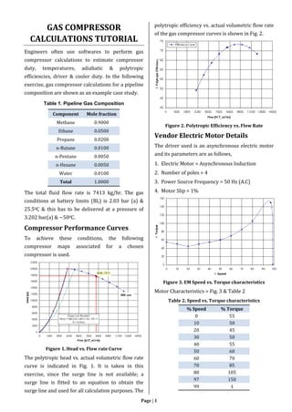
Preliminary System Estimates
Using the compressor data, a process schematic is
proposed as shown in Fig. 4
Figure 4. Proposed CC system Schematic
For the calculations the following is assumed.
1. Pressure drop from suction side Battery limit
(BL) to compressor suction flange = 0.8 bar
2. Pressure drop from discharge flange to
discharge BL = 0.5 bar
3. Pressure drop across suction scrubber is
assumed to be 0 bar. This causes very little
water to be separated & the final gas
composition at the suction flange is shown in
Table 3.
4. Pressure drop across the discharge side air
cooler is taken to be 0.1 bar
Note: Pressure drop data across equipment is
assumed for sample calculation purposes. In reality
pressure drops can be higher.
Table 3. Gas composition After Suction Scrubber
Component
Mass flow Mass Fraction
[kg/hr] [%]
Methane 5823.61 0.7857
Ethane 606.41 0.0818
Propane 355.72 0.0480
n-Butane 234.44 0.0316
n-Pentane 145.51 0.0196
n-Hexane 173.79 0.0234
Water 72.66 0.0098
Total 7412.14 1.0000
Gas Properties at Flange Conditions
The following properties exist at the flange
conditions of the centrifugal compressor.
Table 4. Gas composition after suction separator
Property Value Unit
Gas MW 18.38 kg/kmol
Suction side Density (1) 0.9153 kg/m3
Discharge side Density (2) 2.03 kg/m3
Suction side Heat capacity 2.138 kJ/kg0C
Discharge side Heat capacity 2.474 kJ/kg0C
Z1 at suction flange 0.9964 -
Z2 at discharge flange 0.9964 -
k1 at suction side 1.2740 -
k2 at discharge side 1.2304 -
Calculations
Polytropic Head
From the above data, in order to arrive at a
discharge pressure of 3.202 bar & ~500C at the
discharge battery limit, a pressure drop 0.498 bar
is added to the battery limit to obtain 3.7 bar(a) at
the compressor discharge flange. Similarly, taking
into consideration the pressure losses across the
suction side of 0.9 bar, the suction flange pressure
is taken to be 1.23 bar(a). Taking into account the
temperature drop across the valves on the suction
side, the suction flange temperature is taken to be
250C. Therefore the head produced (Annexure A) is,
1
1
1
1
21
n
n
avg
p
P
P
n
n
MW
RTZ
H (1)
Where,
pH = Polytropic head produced (ft)
avgZ = Average gas compressibility factor (-)
1T =Gas temperature at suction flange (K)
n= Polytropic volume exponent (-)
1
2
P
P
= Pressure ratio at flange conditions (-)
To estimate the polytropic volume exponent, the
following calculation is made.
p
k
k
n
n
11
(2)
Where, p = Polytropic Efficiency](data:image/gif;base64,R0lGODlhAQABAIAAAAAAAP///yH5BAEAAAAALAAAAAABAAEAAAIBRAA7)
Recommended
Recommended
More Related Content
What's hot
What's hot (20)
Similar to Gas Compressor Calculations Tutorial
Similar to Gas Compressor Calculations Tutorial (20)
More from Vijay Sarathy
More from Vijay Sarathy (20)
Recently uploaded
Recently uploaded (20)
Gas Compressor Calculations Tutorial
- 1. Page | 1 GAS COMPRESSOR CALCULATIONS TUTORIAL Engineers often use softwares to perform gas compressor calculations to estimate compressor duty, temperatures, adiabatic & polytropic efficiencies, driver & cooler duty. In the following exercise, gas compressor calculations for a pipeline composition are shown as an example case study. Table 1. Pipeline Gas Composition Component Mole fraction Methane 0.9000 Ethane 0.0500 Propane 0.0200 n-Butane 0.0100 n-Pentane 0.0050 n-Hexane 0.0050 Water 0.0100 Total 1.0000 The total fluid flow rate is 7413 kg/hr. The gas conditions at battery limits (BL) is 2.03 bar (a) & 25.50C & this has to be delivered at a pressure of 3.202 bar(a) & ~500C. Compressor Performance Curves To achieve these conditions, the following compressor maps associated for a chosen compressor is used. Figure 1. Head vs. Flow rate Curve The polytropic head vs. actual volumetric flow rate curve is indicated in Fig. 1. It is taken in this exercise, since the surge line is not available; a surge line is fitted to an equation to obtain the surge line and used for all calculation purposes. The polytropic efficiency vs. actual volumetric flow rate of the gas compressor curves is shown in Fig. 2. Figure 2. Polytropic Efficiency vs. Flow Rate Vendor Electric Motor Details The driver used is an asynchronous electric motor and its parameters are as follows, 1. Electric Motor = Asynchronous Induction 2. Number of poles = 4 3. Power Source Frequency = 50 Hz (A.C) 4. Motor Slip = 1% Figure 3. EM Speed vs. Torque characteristics Motor Characteristics = Fig. 3 & Table 2 Table 2. Speed vs. Torque characteristics % Speed % Torque 0 55 10 50 20 45 30 50 40 55 50 60 60 70 70 85 80 105 97 150 99 1
- 2. Page | 2 Preliminary System Estimates Using the compressor data, a process schematic is proposed as shown in Fig. 4 Figure 4. Proposed CC system Schematic For the calculations the following is assumed. 1. Pressure drop from suction side Battery limit (BL) to compressor suction flange = 0.8 bar 2. Pressure drop from discharge flange to discharge BL = 0.5 bar 3. Pressure drop across suction scrubber is assumed to be 0 bar. This causes very little water to be separated & the final gas composition at the suction flange is shown in Table 3. 4. Pressure drop across the discharge side air cooler is taken to be 0.1 bar Note: Pressure drop data across equipment is assumed for sample calculation purposes. In reality pressure drops can be higher. Table 3. Gas composition After Suction Scrubber Component Mass flow Mass Fraction [kg/hr] [%] Methane 5823.61 0.7857 Ethane 606.41 0.0818 Propane 355.72 0.0480 n-Butane 234.44 0.0316 n-Pentane 145.51 0.0196 n-Hexane 173.79 0.0234 Water 72.66 0.0098 Total 7412.14 1.0000 Gas Properties at Flange Conditions The following properties exist at the flange conditions of the centrifugal compressor. Table 4. Gas composition after suction separator Property Value Unit Gas MW 18.38 kg/kmol Suction side Density (1) 0.9153 kg/m3 Discharge side Density (2) 2.03 kg/m3 Suction side Heat capacity 2.138 kJ/kg0C Discharge side Heat capacity 2.474 kJ/kg0C Z1 at suction flange 0.9964 - Z2 at discharge flange 0.9964 - k1 at suction side 1.2740 - k2 at discharge side 1.2304 - Calculations Polytropic Head From the above data, in order to arrive at a discharge pressure of 3.202 bar & ~500C at the discharge battery limit, a pressure drop 0.498 bar is added to the battery limit to obtain 3.7 bar(a) at the compressor discharge flange. Similarly, taking into consideration the pressure losses across the suction side of 0.9 bar, the suction flange pressure is taken to be 1.23 bar(a). Taking into account the temperature drop across the valves on the suction side, the suction flange temperature is taken to be 250C. Therefore the head produced (Annexure A) is, 1 1 1 1 21 n n avg p P P n n MW RTZ H (1) Where, pH = Polytropic head produced (ft) avgZ = Average gas compressibility factor (-) 1T =Gas temperature at suction flange (K) n= Polytropic volume exponent (-) 1 2 P P = Pressure ratio at flange conditions (-) To estimate the polytropic volume exponent, the following calculation is made. p k k n n 11 (2) Where, p = Polytropic Efficiency
- 3. Page | 3 The specific heat ratio considered is the average specific heat between suction & discharge flange 2522.1 2 2304.1274.1 2 21 kk kavg (3) The polytropic efficiency is taken from Fig. 2, where the efficiency at which the compressor operates is ~71.84%. Therefore substituting in Eq. (2), 3896.17184.0 12522.1 2522.1 1 n n n (4) An alternate way to calculate the polytropic exponent is by using the equation, 1 2 1 2 ln ln P P n (5) Or, 3827.1 9153.0 030.2 ln 23.1 7.3 ln ln ln 1 2 1 2 P P n (6) It is seen that the value of ‘n’ calculated using Eq. (5) is almost equal to the value calculated using Eq. (2). However, since the value of ‘n’ was estimated using a graphically calculated value of p by hand as in Eq. (4), the value obtained using Eq. (6) is considered for calculations. Using the values calculated above, the polytropic head produced is therefore estimated using Eq. (1) as, 1 23.1 7.3 13827.1 3827.1 38.18 67.53635.154529964.09964.0 3827.1 13827.1 pH (7) kgkJftHp /92.17217645m36.57890 (8) Gas Outlet Temperature The gas discharge temperature is calculated (Eq. 9) as (Annexure 2), 2 1 1 1 2 1 2 Z Z P P T T n n (9) Or, 2515.273 9964.0 9964.0 23.1 7.3 3827.1 13827.1 2 T (10) CKT 0 2 2.1314.404 (11) Adiabatic Efficiency The adiabatic efficiency is calculated as follows, 1 1 1 1 1 1 2 1 1 2 k k n n A p P P k k P P n n (12) 0442.1 233.1 2876.1 1 23.1 7.3 12522.1 2522.1 1 23.1 7.3 13827.1 3827.1 2522.1 12522.1 3827.1 13827.1 A p (13) %78.68 0442.1 7182.0 A (14) Inlet Volumetric Flow Rate The inlet volumetric flow rate is calculated as follows, 1 1 m Q (15) hrmQ 3 1 8100 9153.0 7413 (16) Compressor Duty The power absorbed by the compressor to produce a discharge pressure of 3.7 bar(a) is therefore, p p mH P (17) hrkJP 54.1784817 7182.0 741392.172 (18) Or, kWkJP 496sec/8.495 (19) Driver Duty Assuming mechanical losses + margin of 20% of the absorbed power (Actual value to be confirmed by Vendor), the estimated power requirements is 2.1496P (20) rpmatkWP 3000595 (21) In actual practice, the power value selected as shown above may or may not meet the required power to start the compressor from settling out conditions. In such cases a detailed dynamic
- 4. Page | 4 simulation must be performed to check - by how much the compressor loop should be depressurized prior to re-start. The driver rating is to be chosen based on standards such as NEMA or other similar standards. The National Electrical Manufacturer’s Association (NEMA) is an organization that sets the standards for manufacturing of electrical equipment. In the case of electrical induction motors, NEMA sets 4 types of Torque vs Speed Characteristics namely, NEMA A, NEMA B, NEMA C and NEMA D. The characteristics of each type of NEMA motors are depicted below. Figure 5. NEMA Torque vs. Speed Types Table 5. Uses of Different Types of NEMA Motors Among these, NEMA A & NEMA B are the most commonly used due to their high breakdown characteristics and low slip (1% to 5%). For the purpose of this example, the rated motor selected is a 600 kW asynchronous induction electric motor to round–off the calculated value. Cooler Duty To cool the gas from the compressor discharge to say 500C, the cooler duty is calculated as, 32, TTmCQ avgp (22) 15.3234.404 2 220.2473.2 3600 7413 Q (23) hrkJkWQ 6 10414.16.392 (24) Summary The following table shows a summary of the calculated values, Table 6. Summary of Preliminary Estimates Parameter Value Unit Inlet Flange Pressure 1.23 Bar(a) Outlet Flange Pressure 3.70 Bar(a) Polytropic Head 172.92 kJ/kg Discharge Temperature 131.2 0C Adiabatic Efficiency 68.78 % Inlet Volume Flow 8100 Act_m3/hr Compressor Duty 496 kW Driver Rated Duty 600 kW Cooler Duty 392.6 kW Electric Motor Sizing The induction type electric motor available is a 4 pole asynchronous model with a power source at the plant site operating at 50Hz. Therefore, the synchronous speed of the motor is, 4 50120120 Poles frequency N ssynchronou (25) rpmN ssynchronou 1500 (26) From the steady calculations, a 600 kW induction type electric motor has been proposed to be installed. The torque required to sustain the compressor at the rated conditions, the torque required is, kW NT P 100060 2 (27) 14852 100060496 100060 14852 496 T mNTrpm kW (28) mNT 53.3189 (29) Hence the electric motor has to provide a torque of 3189.53 kg-m2 to sustain the compressor at 3000 rpm to meet the rated suction & discharge conditions. The maximum torque that can be provided by the electric motor before it breaks down is calculated at the breakdown torque’s corresponding speed at 97% (Figure 3) rpmN 45.1440148597.0 (30)
- 5. Page | 5 The breakdown torque is estimated as, mNT downbreak 45.59665.1 45.14402 100060600 (31) Hence the power absorbed to generate 5966.5 N-m is 900 kW at a speed of ~1440 rpm during start-up. The inertia offered by the electric motor is calculated by the empirical relationship as, 48.1 0043.0 N P I (32) Where, P = Power [kW] I = Inertia [kg-m2] N = Speed [rpm/1000] Therefore, the inertia offered by the motor is, 48.1 1000 1485 600 0043.0 I (33) 2 97.30 mkgI (34) Therefore the inertia offered by the electric motor (EM) is 30.97 kg-m2. In order to scale up the speed of the compressor, a gearbox is installed. The gear ratio is, 0202.2 1485 3000 GR (35) The gear ratio calculated is 2.0202. Note that the total inertia required to be overcome by the Electric Motor (EM) is the sum of compressor rotor inertia, EM inertia, Gear box Inertia & Gas inertia during start-up & settling out conditions. Annexure A: Compressor Head Derivation The general energy balance for compressors may be written in differential form as gdz c ddhdqdy 2 2 (A.1) Where, y = Specific mass for compressor work input q = Heat flow through the compressor walls [kJ] h = Enthalpy of Gas [kJ/kg] c = Absolute velocity of gas [m/s] g = Gravitational acceleration [m/s2] z = Elevation [m] From the above expression it is seen that the specific mass referenced work input and the heat flow to the compressor is equal to the enthalpy change, change in kinetic energy & static heat difference. Neglecting the velocity terms, static head contributions & the heat input through the walls of the compressor, we obtain, dhdy (A.2) The change in enthalpy of gas is given as, dp dh (A.3) Where, = Density of Gas (kg/m3) p = Pressure of Gas (bara) The specific compressor mass referenced work input is calculated as, 2 1 p p dp y (A.4) The actual work is found by dividing the mass referenced work input by efficiency y W (A.5) Where, W = Actual work applied to the compressor The integral (Eq. A.4) can be solved in ways equivalent to different compression paths such as, 1. Isentropic compression (reversible & adiabatic) - Entropy is constant - 0;0;0 STQ 2. Isothermal compression (reversible & diathermic) - Temperature is constant - 0T 3.Polytropic Compression (irreversible & adiabatic) – Efficiency is constant Isentropic Process As an isothermal process is not feasible in real world applications, this is neglected. However an Isentropic compression can be considered to be an idealistic situation, as it can exist when the process is completely adiabatic & not heat transfer takes place. Therefore for isentropic compression,
- 6. Page | 6 constvp k . (A.6) Where, v p C C k Ratio of Specific Heats Rewriting eq. (A.6), we get const p constp k k 1 (A.7) kkk k kk p p p ppp 1 1 1 1 1 1 1 (A.8) k p p 1 1 1 (A.9) Applying Eq. (A.9) in Eq. (A.4), 2 1 2 1 2 1 1 1 1 1 1 1 1 1 p p k kp p k p p p dpp dp p p dp y (A.10) 2 1 2 1 11 11 1 1 1 1 1 1 1 p p kkp p k k k pp ydpp p y (A.11) 2 1 1 1 1 1 1 p p k k k k k pp y (A.12) Applying Limits & Re-arranging Eq. (A.12) k k k k pp k kp yp k kp y k p p k kk 112 1 12 1 1 1 1 1 1 1 11 (A.13) Taking out P1 as a common term from the brackets, 1 1 1 11 1 2 1 1 1 1 k k k k k k p p k kpp y k (A.14) 1 1 1 1 1 1 2 1 11 1 1 1 2 1 1 1 1 1 k k k k kk k k p p k kp y p p k kpp y k k (A.15) 1 1 1 1 2 1 11 1 k k k k p p k kp y (A.16) 1 1 1 1 2 1 1 k k p p k kp y (A.17) Using Ideal gas equation the pressure & density terms are rewritten using the expression (A.18), nZRTpv (A.18) ZRT p v n (A.19) The above expression gives the density in kmol/m3 & is written in terms of kg/m3 by dividing with molecular weight of the gas. ZRT p MWv M (A.20) Where M = mass of gas MW ZRTp ZRT MWp v M (A.21) Hence for the inlet conditions of the gas into the compressor Eq. (A.21) becomes, MW ZRTp 1 1 1 (A.22) Substituting Eq. (A.22) into Eq. (A.17), 1 1 1 1 21 k k gas p p k k MW ZRT y (A.23) The above expression gives the adiabatic head produced by the compressor & can be written as, aHy (A.24) Where, Ha = Adiabatic Head [m] 1 1 1 1 21 k k gas a p p k k MW ZRT H (A.25) Polytropic Process In all real world compression applications, the polytropic process is predominant & hence the exponent in the ideal gas equation becomes ‘n’ (polytropic volume exponent) which is n1 & Eq. A.6 becomes, constvp n . (A.26) Similarly, performing the above set of calculations using the polytropic exponent, the polytropic head is expressed as follows,
- 7. Page | 7 1 1 1 1 21 n n gas p p p n n MW ZRT H (A.27) The power absorbed by the compressor or the power that is needed at the compressor shaft is estimated as, p gasinp actual mH P , (A.28) Where, p = Polytropic Efficiency [-] gasinm , =Mass flow rate at compressor inlet [kg/s] actualP =Required power at compressor shaft [kW] Annexure B: Compressor Discharge Temperature Derivation The temperature rise at compressor discharge after compression is calculated from Eq. (A.26) as, const p ZRT pconstvp n n . (B.1) Taking the value of gas constant to the right hand side of Eq. (B.1), constZTp nn 1 (B.2) For inlet conditions (suffix 1) to outlet conditions (suffix 2), Eq. (B.2) can be written as, nnnn TZpTZp 22 1 211 1 1 (B.3) nn n n n n TZ TZ p p TZ TZ p p 22 11 1 1 2 22 11 1 1 1 2 (B.4) 1 2 1 1 2 2 1 22 11 1 1 2 Z Z p p T T TZ TZ p p n n n n (B.5) Annexure C: Electric Motor (EM) Implementation in ASPEN HYSYS Dynamics Aspen HYSYS Dynamics provides the option of simulating centrifugal compressors with an Electric Motor (EM). In order to setup the electric motor, the calculations made to arrive at the Electric Motor Input data is entered into Aspen HYSYS Dynamics. Figure 6. Electric Motor in Aspen HYSYS Dynamics References 1. Gas Processors Association. Gas Processors Suppliers Association (1998) P.13-1 to P.13-20 2. HYSYS 2004.2, Operations Guide 2 1 1 1 2 1 2 1 1 2 1 2 1 Z Z p p Z Z p p T T n n n n (B.6) 2 1 1 1 2 1 2 Z Z p p T T n n (B.7) From the above, the discharge temperature at the compressor outlet is calculated from Eq. (B.7).