part2.....

1. Trusses and Frames
The Schematic diagram of a structure on the side of a bridge is drawn in figure 1.
The structure shown in figure 1 is essentially a two-dimensional structure. This is known as a
plane truss. On the other hand, a microwave or mobile phone tower is a three-dimensional
structure. Thus there are two categories of trusses - Plane trusses like on the sides of a bridge
and space trusses like the TV towers. In this course, we will be concentrating on plane trusses in
which the basis elements are stuck together in a plane.
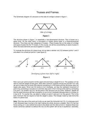
To motivate the structure of a plane truss, let me take a slender rod (12) between points 1 and 2
and attach it to a fixed pin joint at 1 (see figure 2).
Now I put a pin (pin2) at point 2 at the upper end and hang a weight W on it. The question is if we
want to hold the weight at that point, what other minimum supports should we provide? For rods
we are to make only pin joints (We assume everything is in this plane and the structures does not
topple side ways). Since rod (12) tends to turn clockwise, we stop the rightward movement of
point 2 by connecting a rod (23) on it and then stop point 3 from moving to the right by connecting
it to point 1 by another rod (13). All the joints in this structure are pin joints. However, despite all
this the entire structure still has a tendency to turn to turn clockwise because there is a torque on
it due to W. To counter this, we attach a wheel on point 3 and put it on the ground. This is the
bare minimum that we require to hold the weight is place. The triangle made by rods forms the
basis of a plane truss.
Note: One may ask at this point as to why as we need the horizontal rod (13). It is because point
3 will otherwise keep moving to the right making the whole structure unstable. Rod (13) has two
forces acting on it: one vertical force due to the wheel and the other at end 2. However these two
forces cannot be collinear so without the rod (13) the system will not be in equilibrium. Generally,

2. in a truss each joint must be connected to at least three rods or two rods and one external
support.
Let us now analyze forces in the structure that just formed. For simplicity I take the lengths of all
rods to be equal. To get the forces I look at all the forces on each pin and find conditions under
which the pins are in equilibrium. The first thing we note that each rod in equilibrium under the
influence of two forces applied by the pins at their ends. As I discussed in the previous lecture, in
this situation the forces have to be collinear and therefore along the rods only. Thus each rod is
under a tensile or compressive force. Thus rods (12), (23) and (13) experience forces as shown
in figure 3.
Notice that we have taken all the forces to be compressive. If the actual forces are tensile, the
answer will come out to be negative. Let us now look at pin 2. The only forces acting on pin 2 are
F12 due to rod (12) and F23 due to rod (23). Further, it is pulled down by the weight W. Thus forces
acting on pin 2 look like shown in figure 4.
Applying equilibrium condition to pin (2) gives

3. Let us now look at pin 3 (see figure 4). It is in equilibrium under forces F23, normal reaction N and
a horizontal force F13.
Applying equilibrium condition gives
Since the direction of F13 is coming out to be negative, the direction should be opposite to that
assumed. Balance of forces in the vertical direction gives
Thus we see that the weight is held with these three rods. The structure is determinate and it
holds the weight in place.
Even if we replace the pin joints by a small plate (known as gusset plate) with two or three pins in
these, the analysis remains pretty much the same because the pins are so close together that
they hardly create any moment about the joints. Even if the rods are welded together at the joints,
to a great degree of accuracy most of the force is carried longitudinally on the rods, although
some very small (negligible) moment is created by the joints and may be by possible bending of
the rods.
Now we are ready to build a truss and analyze it. We are going to build it by adding more and
more of triangles together. As you can see, when we add these triangles, the member of joints j
and the number of members (rods) m are related as follows:
m = 2j - 3
This makes a truss statically determinate. This is easily understood as follows. First consider the
entire truss as one system. If it is to be statically determinate, there should be only three unknown
forces on it because for forces in a plane there are three equilibrium conditions. Fixing one of its
ends a pin joint and putting the other one on a roller does that (roller also gives the additional
advantage that it can help in adjusting any change in the length of a member due to
deformations). If we wish to determine these external forces and the force in each member of the
truss, the total number of unknowns becomes m + 3. We solve for these unknowns by writing
equilibrium conditions for each pin; there will be 2j such equations. For the system to be
determinate we should have m + 3 = 2j , which is the condition given above. If we add any more
members, these are redundant. On the other hand, less number of members will make the truss
unstable and it will collapse when loaded. This will happen because the truss will not be able to

4. provide the required number of forces for all equilibrium conditions to be satisfied. Statically
determinate trusses are known as simple trusses.
Method of joints: In method of joints, we look at the equilibrium of the pin at the joints. Since the
forces are concurrent at the pin, there is no moment equation and only two equations for
equilibrium viz. . Therefore we start our analysis at a point where one
known load and at most two unknown forces are there. The weight of each member is divided
into two halves and that is supported by each pin. To an extent, we have already alluded to this
method while introducing trusses. Let us illustrate it by two examples.
Example 1: As the first example, I take truss ABCDEF as shown in figure 6 and load it at point E
by 5000N. The length of small members of the truss is 4m and that of the diagonal members is
m. I will now find the forces in each member of this truss assuming them to be weightless.
We take each point to be a pin joint and start balancing forces on each of the pins. Since pin E
has an external load of 5000N one may want to start from there. However, E point has more than
2 unknown forces so we cannot start at E. We therefore first treat the truss as a whole and find
reactions of ground at points A and D because then at points A and D their will remain only two
unknown forces. The horizontal reaction Nx at point A is zero because there is no external
horizontal force on the system. To find N2 I take moment about A to get
which through equation gives

5. In method of joints, let us now start at pin A and balance the various forces. We already anticipate
the direction and show their approximately at A (figure 7). All the angles that the diagonals make
are 45° .
The only equations we now have worry about are the force balance equations.
Keep in mind that the force on the member AB and AF going to be opposite to the forces on the
pin ( Newton 's III
rd
law). Therefore force on member AB is compressive (pushes pin A away)
whereas that on AF is tensile (pulls A towards itself).
Next I consider joint F where force AF is known and two forces BF and FE are unknown. For pint
F
Next I go to point B since now there are only two unknown forces there. At point B

6. Negative sign shows that whereas we have shown FBE to be compressive, it is actually tensile.
Next I consider point C and balance the forces there. I have already anticipated the direction of
the forces and shown FCE to be tensile whereas FCD to be compressive
Next I go to pin D where the normal reaction is N and balance forces there.
Thus forces in various members of the truss have been determined. They are
You may be wondering how we got all the forces without using equations at all joints. Recall that
is how we had obtained the statical determinacy condition. We did not have to use all joints
because already we had treated the system as a whole and had gotten two equations from there.
So one joint - in this case E - does not have to be analyzed. However, given that the truss is
statically determinate, all these forces must balance at point E, where the load has been applied,
also. I will leave this as an exercise for you. Next I ask how the situation would change if each
member of the truss had weight. Suppose each members weighs 500N, then assuming that the
load is divided equally between two pins holding the member the loading of the truss would

7. appear as given in figure 8 (loading due to the weight as shown in red). Except at points A and D
the loading due to the weight is 750N; at the A and D points it is 500N.
Now the external reaction at each end will be.
The extra 2000N can be calculated either from the moment equation or straightaway by realizing
that the new added weight is perfectly symmetric about the centre of the truss and therefore will
be equally divided between the two supports. For balancing forces at other pins, we follow the
same procedure as above, keeping in mind though that each pin now has an external loading due
to the weight of each member. I'll solve for forces in some member of the truss. Looking at pin A,
we get
Next we move to point F and see that the forces are
One can similarly solve for other pins in the truss and I leave that as an exercise for you.

8. Having demonstrated to you the method of joints, we now move on to see the method of sections
that directly gives the force on a desired member of the truss.
Method of sections : As the name suggests in method of sections we make sections through a
truss and then calculate the force in the members of the truss though which the cut is made. For
example, if I take the problem we just solved in the method of joints and make a section S1, S2
(see figure 9), we will be able to determine the forces in members BC, BE and FE by considering
the equilibrium of the portion to the left or the right of the section.
Let me now illustrate this. As in the method of joints, we start by first determining the reactions at
the external support of the truss by considering it as a whole rigid body. In the present particular
case, this gives N at D and N at A. Now let us consider the section of the truss on
the left (see figure 10).

9. Since this entire section is in equilibrium, . Notice that we are
now using all three equations for equilibrium since the forces in individual members are not
concurrent. The direction of force in each member, one can pretty much guess by inspection.
Thus the force in the section of members BE must be pointing down because there is no other
member that can give a downward force to counterbalance N reaction at A. This clearly
tells us that F BE is tensile. Similarly, to counter the torque about B generated by N force at
A, the force on FE should also be from F to E. Thus this force is also tensile. If we next consider
the balance of torque about A, N and FFE do not give any torque about A. So to counter
torque generated by FBE , the force on BC must act towards B, thereby making the force
compressive.
Let us now calculate individual forces. FFE is easiest to calculate. For this we take the moment
about B. This gives
4 × = 4 × F FE
F FE = N
Next we calculate FBE . For this, we use the equation . It gives
Finally to calculate FBC , we can use either the equation about A or
Thus we have determined forces in these three members directly without calculating forces going
from one joint to another joint and have saved a lot of time and effort in the process. The forces
on the right section will be opposite to those on the left sections at points through which the
section is cut. This can be used to check our answer, and I leave it as an exercise for you.
After this illustration let me put down the steps that are taken to solve for forces in members of a
truss by method of sections:

10. 1. Make a cut to divide the truss into section, passing the cut through members where the
force is needed.
2. Make the cut through three member of a truss because with three equilibrium equations
viz. we can solve for a maximum of three forces.
3. Apply equilibrium conditions and solve for the desired forces.
In applying method of sections, ingenuity lies in making a proper. The method after a way of
directly calculating desired force circumventing the hard work involved in applying the method of
joints where one must solve for each joint.
Method of Virtual Work
So far when dealing with equilibrium of bodies/trusses etcetera, our strategy has been to isolate
parts of the system (subsystem) and consider equilibrium of each subsystem under various
forces: the forces that we apply on the system and those that the surfaces, and other elements of
the system apply on the subsystem. As the system size grows, the number of subsystems and
the forces on them becomes very large. The question is can we just focus on the force applied to
get it directly rather than going through each and every subsystem. The method of virtual work
provides such a scheme. In this lecture, I will give you a basic introduction to this method and
solve some examples by applying this method.
Let us take an example: You must have seen a children's toy as shown in figure 1. It is made of
many identical bars connected with each other as shown in the figure. One of the lowest bars is
connected to a fixed pin joint A whereas the other bar is on a pin joint B that can move
horizontally. It is seen that if the toy is extended vertically, it collapses under its own weight. The
question is what horizontal force F should we apply at its upper end so that the structure does not
collapse.

11. To see how many equations do we have to solve in finding F in the structure above, let us take a
simple version of it, made up of only two bars, and ask how much force F do we need to keep it in
equilibrium (see figure 2).
Let each bar be of length l and mass m and let the angle between them be θ. The free-body
diagram of the whole system is shown above. Notice that there are four unknowns - NAx , NAy ,
NBy and F - but only three equilibrium equations: the force equations
and the torque equation
So to solve for the forces we will have to look at individual bars. If we look at individual bars, we
also have to take into account the forces that the pin joining them applies on the bars. This
introduces two more unknowns N1 and N2 into the problem (see figure 3). However, there are
three equations for each bar - or equivalently three equations above and three equations for one
of the bars - so that the total number of equations is also six. Thus we can get all the forces on
the system.

12. The free-body diagrams of the two bars are shown in figure 3. To get three more equations, in
addition to the three above, we can consider equilibrium of any of the two bars. In the present
case, doing this for the bar pinned at B appears to be easy so we will consider that bar. The force
equations for this bar give
And taking torque about B , taking N1 = 0 , gives
This then leads to (from the force equation above)
Substituting these in the three equilibrium equations obtained for the entire system gives
Looking at the answers carefully reveals that all we are doing by applying the force F is to make
sure that the bar at pin-joint A is in equilibrium. This bar then keeps the bar at joint B in
equilibrium by applying on it a force equal to its weight at its centre of gravity.
The question that arises is if we have many of these bars in a folding toy shown in figure 1, how
would we calculate F ? This is where the method of virtual work, to be developed in this lecture,
would come in handy. We will solve this problem later using the method of virtual work. So let us
now describe the method. First we introduce the terminology to be employed in this method.
1. Degrees of freedom: This is the number of parameters required to describe the system. For
example a free particle has three degrees of freedom because we require x, y , and z to describe
its position. On the other hand if it is restricted to move in a plane, its degrees of freedom an only
two. In the mechanism that we considered above, there is only one degree of freedom because

13. angle θ between the bars is sufficient to describe the system. Degrees of freedom are reduced by
the constraints that are put on the possible motion of a system. These are discussed below.
2. Constraints and constraint forces: Constraints and those conditions that we put on the
movement of a system so that its motion gets restricted. In other words, a constraint reduces the
degrees of freedom of a system. Constraint forces are the forces that are applied on a system to
enforce a constraint. Let us understand these concepts through some examples.
A particle in free space has three degrees of freedom. However, if we put it on a plane horizontal
surface without applying any force in the vertical direction, its motion is restricted to that plane.
Thus now it has only two degrees of freedom. So the constraint in this case is that the particle
moves on the horizontal surface only. The corresponding force of constraint is the normal
reaction provided by the surface.
As the second example, let us take the case of a vertical pendulum oscillating in a plane (see
figure 5). Thus its degrees of freedom would be two if there were no more constraints on its
motion. However, the bob of a pendulum is constrained to move in such a way that its distance
from the pivot point remains fixed. We have thus introduced one more constraint on its motion
and therefore the degrees of freedom are reduced by one; a pendulum oscillating in a plane has
only one degree of freedom. The angle from the equilibrium position is therefore sufficient to
describe a plane pendulum's motion fully. How about the force of constraint in this case? The
constraint, that the distance of the bob from the pivot point remains fixed, is ensured by the
tension in the string. The tension in the string is therefore the force of constraint.

14. Let us now consider the folding toy shown in figure 1. This structure, although made of many
moving bars, has only one degree of freedom because the bars are constrained to move in a very
specific way. Thus from a large number of degrees of freedom for these bars, all of them except
one are eliminated by the constraints. As such the number of constraints, and therefore the
number of constraint forces, is very large. The constraint forces are the reactions at the supports
A and B and the forces applied by the pins holding the bars together. It is because of these forces
that the system is restricted in its motion.
I would like you to note one thing interesting in the examples considered above: if the system
moves the constraint forces do not do any work on it. In the case of a particle moving on a plane,
the motion is perpendicular to the normal reaction so it does no work on the particle. In the
pendulum the motion of the bob is also perpendicular to the tension in the string which is the
force of constraint. Thus no work is done on the bob by the constraint force. The case of the toy
in figure 1 is quite interesting. In the structure point A does not move and the motion of point B is
perpendicular to the reaction force at B. Thus there is no work done by the reaction forces at
these points. On the other hand, the constraint forces due to pins connecting two bars are equal
and opposite on each bar. But the points on the bar where these forces act (the points where the
pin joints are) have the same displacement for each bar so that the net work done by the
constraint forces vanishes.
3. Virtual displacement: Given a system in equilibrium, its virtual displacement is imagined as
follows: Move the system slightly away from its equilibrium position arbitrarily but consistent with
the constraints. This represents a virtual displacement of the system. Note the emphasis on the
word imagined. This is because a virtual displacement is not caused by the applied forces. Rather
it is the difference between the equilibrium position of the system and an imagined position -
consistent with the constraints - of the system slightly away from the equilibrium. For example in
the case of a pendulum under equilibrium at an angle θ under a force P (see figure 6), virtual
displacement would be increasing the angle from θ to ( θ + Δθ) keeping the distance of the bob
from the pivot unchanged. On the other hand, moving the bob with a component in the direction
of the string is not a virtual displacement because it will not be consistent with the constraint.
Virtual displacement is denoted by to distinguish it from a real displacement .

15. 4. Virtual work: The work done by any force during a virtual displacement is called virtual
work. It is denoted by . Thus
Note that our previous observation, that work done by a constraint force is usually zero, implies
that virtual work done by a constraint force is also zero. Also keep in mind that in calculating the
work done by the force , represents the displacement of the point where the force
is being applied.
With these definitions we are now ready to state the principle of virtual work. It is based on the
assumption that virtual work done by a constraint force is zero. The principle of virtual work states
that " The necessary and sufficient condition for equilibrium of a mechanical system without
friction is that the virtual work done by the externally applied forces is zero ". Let us see how it
arises. For a system in equilibrium, each particle in the system is in equilibrium under the
influence of externally applied forces and the forces of constraints. Then for the i
th
particle
Therefore

16. But we have already seen that for individual particles and for a system
composed of many subsystems , that is the net virtual work done by
constraint forces is zero. This means that the total virtual work done by the external forces
vanishes, i.e.
This is the necessary part of the proof. The condition is also sufficient condition. This is proved by
showing that if the body is not in equilibrium, the virtual work done by the external forces does not
vanish for all arbitrary virtual displacements (consistent with the constraints). If the body is not in
equilibrium, it will move in the direction of the net force on each particle. During this real
displacement the work don by the force on the ith
particle will be positive i.e.
Now we can choose this real displacement to be the virtual displacement and find that when the
body is not in equilibrium, all virtual displacements consistent with the constraints will not give
zero virtual work. Thus when the system is not in equilibrium
Assuming again that the net work done by the constraint forces is zero, we get that for a body not
in equilibrium
This implies that when the virtual work done by external forces vanishes, the system must be in
equilibrium. This proves the sufficiency part of the condition. We now solve some examples to
illustrate how the method of virtual work is applied.
Example 1: A pendulum in equilibrium as shown in figure 5. We show the coordinates of the bob
in the figure 7 below.

17. If the pendulum is give a virtual displacement i.e.
By the principle of virtual work, the total virtual work done by the external forces vanishes at
equilibrium. So the equilibrium is described by
giving
Which is the same answer as obtained earlier.
Example 2: This is the problem involving two crossed bars as shown in figure 2. We wish to
calculate the force F required to keep the system in equilibrium using the principle of virtual work.
To apply the principle of virtual work, imagine a virtual displacement consistent with the
constraint. The only displacement possible - because of only one degree of freedom - is that
. From figure 2 it is clear that the external forces on the system are F and 2mg
(weight of the bars).

18. As θ increased to θ + Δθ , the point where the bars cross moves down by a distance (see figure
8)
and the point when F is applied moves to the right by a distance
To calculate the net virtual work done, I remind you that work by a force is calculated by taking
the dot product , where represents the displacement of the point where the force is
being applied. Thus the virtual work in the present case is
For equilibrium we equate this to zero to get
which is the same result as obtained earlier.
So you see in both these examples that by applying the method of virtual work, we have
bypassed calculating the constraint forces completely and that is what makes the method easy to
implement in large systems. The way to learn the method well is to practice as many problems as
possible. I will now solve some examples to demonstrate the usefulness of the method for large

19. system. To start with let us take the example which we gave in the beginning - that of toy with
made with bars.
Example 3: If there are N crossings in the folding toy shown in figure 9, what is the force required
to keep the system in equilibrium?
Again the degree of freedom = 1. The variable we use to describe the position of the mechanism
is the angle between the bars i.e. θ. As the angle θ is changed to (θ+ Δθ), the upper end of the
bar where force F is applied moves in the direction opposite to the force by
Thus the virtual work done by F is
On the other hand, the first crossing moves down by
The second crossing by

20. and the Nth crossing moves down by
All these displacements are in the same direction as the force = 2mg at each of the bar crossings.
Thus the virtual work done by the weight of the mechanism is
This gives a total virtual work done by the external forces to be
Equating this to zero for equilibrium gives
For N = 1 the answer matches with that obtained in the case of only two bars in example 2 above.
For larger N , the force required to keep equilibrium goes up by a factor of N
2
.
Example 4: A 6m long electric pole of weight W starts falling to one side during rains. It is kept
from falling by tying a strong rope at its centre of gravity (assumed to be right in the middle of the
pole) and securing the other end of the rope on ground. All the relevant distances are given in
figure 10. Assume that the lower end of the pole is like a pin joint. Under these conditions we
want to find the tension in the rope using the method of virtual work.

21. In this problem also there is only one degree of freedom θ. The constraint is that the pole can
only rotate about the assumed pin joint at the ground. The constraint forces are the reactions at
the ground and do no work on the pole when it rotates. There is also the constraint of the rigidity
of the pole. Extend forces are W and T. By principle of virtual work when θ is changed to ( θ + Δ θ
) , the total virtual work vanishes. If the centre of gravity moves up by Δy and to the left by Δx as θ
is increased to ( θ + Δθ ) , the virtual work done is
which, when equated to zero, gives
From the figure it is easy to see that
and (only the magnitude)
Substituting these in the expression for the tension gives

22. Stress and strain analysis
Engineering science is usually subdivided into number of topics such as
1. Solid Mechanics
2. Fluid Mechanics
3. Heat Transfer
4. Properties of materials and soon Although there are close links between them in terms of the physical
principles involved and methods of analysis employed.
The solid mechanics as a subject may be defined as a branch of applied mechanics that deals with
behaviours of solid bodies subjected to various types of loadings. This is usually subdivided into further two
streams i.e Mechanics of rigid bodies or simply Mechanics and Mechanics of deformable solids.
The mechanics of deformable solids which is branch of applied mechanics is known by several names i.e.
strength of materials, mechanics of materials etc.
Mechanics of rigid bodies:
The mechanics of rigid bodies is primarily concerned with the static and dynamic behaviour under external
forces of engineering components and systems which are treated as infinitely strong and undeformable
Primarily we deal here with the forces and motions associated with particles and rigid bodies.
Mechanics of deformable solids :
Mechanics of solids:
The mechanics of deformable solids is more concerned with the internal forces and associated changes in
the geometry of the components involved. Of particular importance are the properties of the materials used,
the strength of which will determine whether the components fail by breaking in service, and the stiffness of
which will determine whether the amount of deformation they suffer is acceptable. Therefore, the subject of
mechanics of materials or strength of materials is central to the whole activity of engineering design. Usually
the objectives in analysis here will be the determination of the stresses, strains, and deflections produced by
loads. Theoretical analyses and experimental results have an equal roles in this field.
Analysis of stress and strain :
Concept of stress : Let us introduce the concept of stress as we know that the main problem of
engineering mechanics of material is the investigation of the internal resistance of the body, i.e. the nature of
forces set up within a body to balance the effect of the externally applied forces.
The externally applied forces are termed as loads. These externally applied forces may be due to any one of
the reason.

23. (i) due to service conditions
(ii) due to environment in which the component works
(iii) through contact with other members
(iv) due to fluid pressures
(v) due to gravity or inertia forces.
As we know that in mechanics of deformable solids, externally applied forces acts on a body and body
suffers a deformation. From equilibrium point of view, this action should be opposed or reacted by internal
forces which are set up within the particles of material due to cohesion.
These internal forces give rise to a concept of stress. Therefore, let us define a stress Therefore, let us
define a term stress
Stress:
Let us consider a rectangular bar of some cross – sectional area and subjected to some load or force (in
Newtons )
Let us imagine that the same rectangular bar is assumed to be cut into two halves at section XX. The each
portion of this rectangular bar is in equilibrium under the action of load P and the internal forces acting at the
section XX has been shown
Now stress is defined as the force intensity or force per unit area. Here we use a symbol  to represent the
stress.

24. Where A is the area of the X – section
Here we are using an assumption that the total force or total load carried by the rectangular bar is uniformly
distributed over its cross – section.
But the stress distributions may be for from uniform, with local regions of high stress known as stress
concentrations.
If the force carried by a component is not uniformly distributed over its cross – sectional area, A, we must
consider a small area, ‘A' which carries a small load P, of the total force ‘P', Then definition of stress is
As a particular stress generally holds true only at a point, therefore it is defined mathematically as
Units :
The basic units of stress in S.I units i.e. (International system) are N / m2
(or Pa)
MPa = 106
Pa
GPa = 109
Pa
KPa = 103
Pa
Some times N / mm2
units are also used, because this is an equivalent to MPa. While US customary unit is
pound per square inch psi.
TYPES OF STRESSES :
only two basic stresses exists : (1) normal stress and (2) shear shear stress. Other stresses either are
similar to these basic stresses or are a combination of these e.g. bending stress is a combination tensile,
compressive and shear stresses. Torsional stress, as encountered in twisting of a shaft is a shearing stress.
Let us define the normal stresses and shear stresses in the following sections.
Normal stresses : We have defined stress as force per unit area. If the stresses are normal to the areas
concerned, then these are termed as normal stresses. The normal stresses are generally denoted by a
Greek letter (  )

25. This is also known as uniaxial state of stress, because the stresses acts only in one direction however, such
a state rarely exists, therefore we have biaxial and triaxial state of stresses where either the two mutually
perpendicular normal stresses acts or three mutually perpendicular normal stresses acts as shown in the
figures below :
Tensile or compressive stresses :
The normal stresses can be either tensile or compressive whether the stresses acts out of the area or into
the area

26. Bearing Stress : When one object presses against another, it is referred to a bearing stress ( They are in
fact the compressive stresses ).
Shear stresses :
Let us consider now the situation, where the cross – sectional area of a block of material is subject to a
distribution of forces which are parallel, rather than normal, to the area concerned. Such forces are
associated with a shearing of the material, and are referred to as shear forces. The resulting force interistes
are known as shear stresses.
The resulting force intensities are known as shear stresses, the mean shear stress being equal to
Where P is the total force and A the area over which it acts.
As we know that the particular stress generally holds good only at a point therefore we can define shear
stress at a point as
The greek symbol  ( tau ) ( suggesting tangential ) is used to denote shear stress.

27. However, it must be borne in mind that the stress ( resultant stress ) at any point in a body is basically
resolved into two components  and  one acts perpendicular and other parallel to the area concerned, as it
is clearly defined in the following figure.
The single shear takes place on the single plane and the shear area is the cross - sectional of the rivett,
whereas the double shear takes place in the case of Butt joints of rivetts and the shear area is the twice of
the X - sectional area of the rivett.
ANALYSIS OF STERSSES
General State of stress at a point :
Stress at a point in a material body has been defined as a force per unit area. But this definition is some
what ambiguous since it depends upon what area we consider at that point. Let us, consider a point ‘q' in the
interior of the body
Let us pass a cutting plane through a pont 'q' perpendicular to the x - axis as shown below

28. The corresponding force components can be shown like this
dFx = xx. dax
dFy = xy. dax
dFz = xz. dax
where dax is the area surrounding the point 'q' when the cutting plane  r
is to x - axis.
In a similar way it can be assummed that the cutting plane is passed through the point 'q' perpendicular to
the y - axis. The corresponding force components are shown below
The corresponding force components may be written as
dFx = yx. day
dFy = yy. day
dFz = yz. day
where day is the area surrounding the point 'q' when the cutting plane 
r
is to y - axis.
In the last it can be considered that the cutting plane is passed through the point 'q' perpendicular to the z -
axis.

29. The corresponding force components may be written as
dFx = zx. daz
dFy = zy. daz
dFz = zz. daz
where daz is the area surrounding the point 'q' when the cutting plane 
r
is to z - axis.
Thus, from the foregoing discussion it is amply clear that there is nothing like stress at a point 'q' rather we
have a situation where it is a combination of state of stress at a point q. Thus, it becomes imperative to
understand the term state of stress at a point 'q'. Therefore, it becomes easy to express astate of stress by
the scheme as discussed earlier, where the stresses on the three mutually perpendiclar planes are labelled
in the manner as shown earlier. the state of stress as depicted earlier is called the general or a triaxial state
of stress that can exist at any interior point of a loaded body.
Before defining the general state of stress at a point. Let us make overselves conversant with the notations
for the stresses.
We have already chosen to distinguish between normal and shear stress with the help of symbols 
and  .
Cartesian - co-ordinate system
In the Cartesian co-ordinates system, we make use of the axes, X, Y and Z
Let us consider the small element of the material and show the various normal stresses acting the faces

30. Thus, in the Cartesian co-ordinates system the normal stresses have been represented by x, yand z.
Cylindrical - co-ordinate system
In the Cylindrical - co-ordinate system we make use of co-ordinates r,  and Z.
Thus, in the Cylindrical co-ordinates system, the normal stresses i.e components acting over a element is
being denoted by r, and z.
Sign convention : The tensile forces are termed as ( +ve ) while the compressive forces are termed as
negative ( -ve ).
First sub – script : it indicates the direction of the normal to the surface.
Second subscript : it indicates the direction of the stress.
It may be noted that in the case of normal stresses the double script notation may be dispensed with as the
direction of the normal stress and the direction of normal to the surface of the element on which it acts is the
same. Therefore, a single subscript notation as used is sufficient to define the normal stresses.
Shear Stresses : With shear stress components, the single subscript notation is not practical, because such
stresses are in direction parallel to the surfaces on which they act. We therefore have two directions to
specify, that of normal to the surface and the stress itself. To do this, we stress itself. To do this, we attach
two subscripts to the symbol ' ' , for shear stresses.
In cartesian and polar co-ordinates, we have the stress components as shown in the figures.
xy , yx , yz , zy , zx , xz
r , r , z , z ,zr , rz

31. So as shown above, the normal stresses and shear stress components indicated on a small element of
material seperately has been combined and depicted on a single element. Similarly for a cylindrical co-
ordinate system let us shown the normal and shear stresses components separately.
Now let us combine the normal and shear stress components as shown below :

32. Now let us define the state of stress at a point formally.
State of stress at a point :
By state of stress at a point, we mean an information which is required at that point such that it remains
under equilibrium. or simply a general state of stress at a point involves all the normal stress components,
together with all the shear stress components as shown in earlier figures.
Therefore, we need nine components, to define the state of stress at a point
x xy xz
y yx yz
z zx zy
If we apply the conditions of equilibrium which are as follows:
 Fx = 0 ;  M x = 0
 Fy = 0 ;  M y = 0
 Fz = 0 ;  M z = 0
Then we get
xy = yx
yz = zy
zx = xy
Then we will need only six components to specify the state of stress at a point i.e
x , y, z , xy , yz , zx

33. Now let us define the concept of complementary shear stresses.
Complementary shear stresses:
The existence of shear stresses on any two sides of the element induces complementary shear stresses on
the other two sides of the element to maintain equilibrium.
on planes AB and CD, the shear stress  acts. To maintain the static equilibrium of this element, on planes
AD and BC, ' should act, we shall see that ' which is known as the complementary shear stress would
come out to equal and opposite to the. Let us prove this thing for a general case as discussed below:
The figure shows a small rectangular element with sides of length x, y parallel to x and y directions. Its
thickness normal to the plane of paper is z in z – direction. All nine normal and shear stress components
may act on the element, only those in x and y directions are shown.
Sign convections for shear stresses:
Direct stresses or normal stresses
- tensile +ve
- compressive –ve
Shear stresses:
- tending to turn the element C.W +ve.
- tending to turn the element C.C.W – ve.

34. The resulting forces applied to the element are in equilibrium in x and y direction. ( Although other normal
and shear stress components are not shown, their presence does not affect the final conclusion ).
Assumption : The weight of the element is neglected.
Since the element is a static piece of solid body, the moments applied to it must also be in equilibrium. Let
‘O' be the centre of the element. Let us consider the axis through the point ‘O'. the resultant force associated
with normal stresses x and y acting on the sides of the element each pass through this axis, and therefore,
have no moment.
Now forces on top and bottom surfaces produce a couple which must be balanced by the forces on left and
right hand faces
Thus,
yx .  x .  z .  y = xy .  x .  z .  y
In other word, the complementary shear stresses are equal in magnitude. The same form of relationship can
be obtained for the other two pair of shear stress components to arrive at the relations
Analysis of Stresses:
Consider a point ‘q' in some sort of structural member like as shown in figure below. Assuming that at point
exist. ‘q' a plane state of stress exist. i.e. the state of state stress is to describe by a parameters x, y and
xy These stresses could be indicate a on the two dimensional diagram as shown below:

35. This is a commen way of representing the stresses. It must be realize a that the material is unaware of what
we have called the x and y axes. i.e. the material has to resist the loads irrespective less of how we wish to
name them or whether they are horizontal, vertical or otherwise further more, the material will fail when the
stresses exceed beyond a permissible value. Thus, a fundamental problem in engineering design is to
determine the maximum normal stress or maximum shear stress at any particular point in a body. There is
no reason to believe apriori that x, y and xy are the maximum value. Rather the maximum stresses may
associates themselves with some other planes located at ‘'. Thus, it becomes imperative to determine the
values of  and. In order tto achieve this let us consider the following.
Shear stress:
If the applied load P consists of two equal and opposite parallel forces not in the same line, than there is a
tendency for one part of the body to slide over or shear from the other part across any section LM. If the
cross section at LM measured parallel to the load is A, then the average value of shear stress  = P/A . The
shear stress is tangential to the area over which it acts.
If the shear stress varies then at a point then  may be defined as

36. Complementary shear stress:
Let ABCD be a small rectangular element of sides x, y and z perpendicular to the plane of paper let there be
shear stress acting on planes AB and CD
It is obvious that these stresses will from a couple (  . xz )y which can only be balanced by tangential forces
on planes AD and BC. These are known as complementary shear stresses. i.e. the existence of shear
stresses on sides AB and CD of the element implies that there must also be complementary shear stresses
on to maintain equilibrium.
Let ' be the complementary shear stress induced on planes
AD and BC. Then for the equilibrium ( . xz )y = ' ( yz )x
 = '
Thus, every shear stress is accompanied by an equal complementary shear stress.
Stresses on oblique plane: Till now we have dealt with either pure normal direct stress or pure shear
stress. In many instances, however both direct and shear stresses acts and the resultant stress across any
section will be neither normal nor tangential to the plane.
A plane stse of stress is a 2 dimensional stae of stress in a sense that the stress components in one
direction are all zero i.e
z = yz = zx = 0
examples of plane state of stress includes plates and shells.
Consider the general case of a bar under direct load F giving rise to a stress y vertically

37. The stress acting at a point is represented by the stresses acting on the faces of the element enclosing the
point.
The stresses change with the inclination of the planes passing through that point i.e. the stress on the faces
of the element vary as the angular position of the element changes.
Let the block be of unit depth now considering the equilibrium of forces on the triangle portion ABC
Resolving forces perpendicular to BC, gives
.BC.1 = ysin . AB . 1
but AB/BC = sin or AB = BCsin
Substituting this value in the above equation, we get
.BC.1 = ysin . BCsin . 1 or (1)
Now resolving the forces parallel to BC
.BC.1 = y cos . ABsin . 1
again AB = BCcos
.BC.1 = ycos . BCsin . 1 or = ysincos
(2)
If  = 90
0
the BC will be parallel to AB and  = 0, i.e. there will be only direct stress or normal stress.
By examining the equations (1) and (2), the following conclusions may be drawn

38. (i) The value of direct stress  is maximum and is equal to y when  = 900
.
(ii) The shear stress  has a maximum value of 0.5 y when  = 450
(iii) The stresses  and  are not simply the resolution of y
Material subjected to pure shear:
Consider the element shown to which shear stresses have been applied to the sides AB and DC
Complementary shear stresses of equal value but of opposite effect are then set up on the sides AD and BC
in order to prevent the rotation of the element. Since the applied and complementary shear stresses are of
equal value on the x and y planes. Therefore, they are both represented by the symbol xy.
Now consider the equilibrium of portion of PBC
Assuming unit depth and resolving normal to PC or in the direction of 
.PC.1 =xy.PB.cos.1+xy.BC.sin.1
= xy.PB.cos + xy.BC.sin
Now writing PB and BC in terms of PC so that it cancels out from the two sides
PB/PC = sin BC/PC = cos
.PC.1 = xy.cossinPC+ xy.cos.sinPC

39.  = 2xysincos
 = xy.2.sincos
(1)
Now resolving forces parallel to PC or in the direction .then xyPC . 1 =xy . PBsin xy . BCcos
ve sign has been put because this component is in the same direction as that of .
again converting the various quantities in terms of PC we have
xyPC . 1 =xy . PB.sin
2
 xy . PCcos
2

= [xy (cos
2
 sin
2
) ]
= xycos2or (2)
the negative sign means that the sense of  is opposite to that of assumed one. Let us examine the
equations (1) and (2) respectively
From equation (1) i.e,
 = xy sin2
The equation (1) represents that the maximum value of  isxy when  = 45
0
.
Let us take into consideration the equation (2) which states that
 =xy cos2
It indicates that the maximum value of  isxy when  = 0
0
or 90
0
. it has a value zero when  = 45
0
.
From equation (1) it may be noticed that the normal component  has maximum and minimum values of
+xy (tension) and xy (compression) on plane at ± 45
0
to the applied shear and on these planes the
tangential component  is zero.
Hence the system of pure shear stresses produces and equivalent direct stress system, one set
compressive and one tensile each located at 450
to the original shear directions as depicted in the figure
below:

40. Material subjected to two mutually perpendicular direct stresses:
Now consider a rectangular element of unit depth, subjected to a system of two direct stresses both tensile,
x and yacting right angles to each other.
for equilibrium of the portion ABC, resolving perpendicular to AC
 . AC.1 = y sin  . AB.1 + x cos  . BC.1
converting AB and BC in terms of AC so that AC cancels out from the sides
 = y sin
2
 + xcos
2

Futher, recalling that cos
2
 sin
2
 = cos2 or (1  cos2)/2 = sin
2

Similarly (1 + cos2)/2 = cos
2
q

41. Hence by these transformations the expression for  reduces to
= 1/2y (1  cos2) + 1/2x (1 + cos2)
On rearranging the various terms we get
(3)
Now resolving parallal to AC
sq.AC.1= xy..cos.AB.1+xy.BC.sin.1
The – ve sign appears because this component is in the same direction as that of AC.
Again converting the various quantities in terms of AC so that the AC cancels out from the two sides.
(4)
Conclusions :
The following conclusions may be drawn from equation (3) and (4)
(i) The maximum direct stress would be equal to x or y which ever is the greater, when  = 0
0
or 90
0
(ii) The maximum shear stress in the plane of the applied stresses occurs when = 45
0
Material subjected to combined direct and shear stresses:
Now consider a complex stress system shown below, acting on an element of material.
The stresses x and y may be compressive or tensile and may be the result of direct forces or as a result of
bending.The shear stresses may be as shown or completely reversed and occur as a result of either shear
force or torsion as shown in the figure below:

42. As per the double subscript notation the shear stress on the face BC should be notified as yx , however, we
have already seen that for a pair of shear stresses there is a set of complementary shear stresses
generated such that yx = xy
By looking at this state of stress, it may be observed that this state of stress is combination of two different
cases:
(i) Material subjected to pure stae of stress shear. In this case the various formulas deserved are as follows
 = yx sin2
 = yx cos 2
(ii) Material subjected to two mutually perpendicular direct stresses. In this case the various formula's
derived are as follows.
To get the required equations for the case under consideration,let us add the respective equations for the
above two cases such that
These are the equilibrium equations for stresses at a point. They do not depend on material proportions and
are equally valid for elastic and inelastic behaviour
This eqn gives two values of 2 that differ by 180
0
.Hence the planes on which maximum and minimum
normal stresses occurate 90
0
apart.

43. From the triangle it may be determined
Substituting the values of cos2 and sin2 in equation (5) we get

44. This shows that the values oshear stress is zero on the principal planes.
Hence the maximum and minimum values of normal stresses occur on planes of zero shearing stress. The
maximum and minimum normal stresses are called the principal stresses, and the planes on which they act
are called principal plane the solution of equation
will yield two values of 2 separated by 1800
i.e. two values of  separated by 900
.Thus the two principal
stresses occur on mutually perpendicular planes termed principal planes.

45. Therefore the two – dimensional complex stress system can now be reduced to the equivalent system of
principal stresses.
Let us recall that for the case of a material subjected to direct stresses the value of maximum shear stresses
Therefore,it can be concluded that the equation (2) is a negative reciprocal of equation (1) hence the roots
for the double angle of equation (2) are 90
0
away from the corresponding angle of equation (1).

46. This means that the angles that angles that locate the plane of maximum or minimum shearing stresses
form angles of 45
0
with the planes of principal stresses.
Futher, by making the triangle we get
Because of root the difference in sign convention arises from the point of view of locating the planes on
which shear stress act. From physical point of view these sign have no meaning.
The largest stress regard less of sign is always know as maximum shear stress.
Principal plane inclination in terms of associated principal stress:
We know that the equation
yields two values of q i.e. the inclination of the two principal planes on which the principal stresses s1 and s2
act. It is uncertain,however, which stress acts on which plane unless equation.
is used and observing which one of the two principal
stresses is obtained.
Alternatively we can also find the answer to this problem in the following manner

47. Consider once again the equilibrium of a triangular block of material of unit depth, Assuming AC to be a
principal plane on which principal stresses p acts, and the shear stress is zero.
Resolving the forces horizontally we get:
x .BC . 1 + xy .AB . 1 = p . cos . AC dividing the above equation through by BC we get
ANALYSIS OF STRAINS
CONCEPT OF STRAIN
Concept of strain : if a bar is subjected to a direct load, and hence a stress the bar will change in length. If
the bar has an original length L and changes by an amount L, the strain produce is defined as follows:
Strain is thus, a measure of the deformation of the material and is a nondimensional Quantity i.e. it has no
units. It is simply a ratio of two quantities with the same unit.

48. Since in practice, the extensions of materials under load are very very small, it is often convenient to
measure the strain in the form of strain x 10-6
i.e. micro strain, when the symbol used becomes .
Sign convention for strain:
Tensile strains are positive whereas compressive strains are negative. The strain defined earlier was known
as linear strain or normal strain or the longitudinal strain now let us define the shear strain.
Definition: An element which is subjected to a shear stress experiences a deformation as shown in the
figure below. The tangent of the angle through which two adjacent sides rotate relative to their initial position
is termed shear strain. In many cases the angle is very small and the angle it self is used, ( in radians ),
instead of tangent, so that  =  AOB -  A'OB' =
Shear strain: As we know that the shear stresses acts along the surface. The action of the stresses is to
produce or being about the deformation in the body consider the distortion produced b shear sheer stress on
an element or rectangular block
This shear strain or slide is and can be defined as the change in right angle. or The angle of deformation 
is then termed as the shear strain. Shear strain is measured in radians & hence is non – dimensional i.e. it
has no unit.So we have two types of strain i.e. normal stress & shear stresses.
Hook's Law :

49. A material is said to be elastic if it returns to its original, unloaded dimensions when load is removed.
Hook's law therefore states that
Stress ( )  strain( )
Modulus of elasticity : Within the elastic limits of materials i.e. within the limits in which Hook's law applies,
it has been shown that
Stress / strain = constant
This constant is given by the symbol E and is termed as the modulus of elasticity or Young's modulus of
elasticity
Thus
The value of Young's modulus E is generally assumed to be the same in tension or compression and for
most engineering material has high, numerical value of the order of 200 GPa
Poisson's ratio: If a bar is subjected to a longitudinal stress there will be a strain in this direction equal to
E . There will also be a strain in all directions at right angles to  . The final shape being shown by the dotted
lines.
It has been observed that for an elastic materials, the lateral strain is proportional to the longitudinal strain.
The ratio of the lateral strain to longitudinal strain is known as the poison's ratio .
Poison's ratio ( ) =  lateral strain / longitudinal strain
For most engineering materials the value of  his between 0.25 and 0.33.
Three – dimensional state of strain : Consider an element subjected to three mutually perpendicular
tensile stresses x , yand z as shown in the figure below.

50. If y and z were not present the strain in the x direction from the basic definition of Young's modulus of
Elasticity E would be equal to
x= x/ E
The effects of y and z in x direction are given by the definition of Poisson's ratio ‘  ' to be equal as y/
E and z/ E
The negative sign indicating that if yand z are positive i.e. tensile, these they tend to reduce the strain in x
direction thus the total linear strain is x direction is given by
Principal strains in terms of stress:
In the absence of shear stresses on the faces of the elements let us say that x , y , z are in fact the
principal stress. The resulting strain in the three directions would be the principal strains.
i.e. We will have the following relation.
For Two dimensional strain: system, the stress in the third direction becomes zero i.e z = 0 or 3 = 0
Although we will have a strain in this direction owing to stresses 1& 2 .

51. Hence the set of equation as described earlier reduces to
Hence a strain can exist without a stress in that direction
Hydrostatic stress : The term Hydrostatic stress is used to describe a state of tensile or compressive
stress equal in all directions within or external to a body. Hydrostatic stress causes a change in volume of a
material, which if expressed per unit of original volume gives a volumetric strain denoted byv. So let us
determine the expression for the volumetric strain.
Volumetric Strain:

52. Consider a rectangle solid of sides x, y and z under the action of principal stresses 1 , 2 , 3 respectively.
Then 1 , 2 , and 3 are the corresponding linear strains, than the dimensions of the rectangle becomes
( x + 1 . x ); ( y + 2 . y ); ( z + 3 . z )
hence
the
ALITER : Let a cuboid of material having initial sides of Length x, y and z. If under some load system, the
sides changes in length by dx, dy, and dz then the new volume ( x + dx ) ( y + dy ) ( z +dz )
New volume = xyz + yzdx + xzdy + xydz
Original volume = xyz
Change in volume = yzdx +xzdy + xydz
Volumetric strain = ( yzdx +xzdy + xydz ) / xyz = x+ y+ z
Neglecting the products of epsilon's since the strains are sufficiently small.
Volumetric strains in terms of principal stresses:
As we know that
Strains on an oblique plane
(a) Linear strain

53. Consider a rectangular block of material OLMN as shown in the xy plane. The strains along ox and oy are x
and y , and xy is the shearing strain.
Then it is required to find an expression for , i.e the linear strain in a direction inclined at  to OX, in terms
of x ,y , xy and .
Let the diagonal OM be of length 'a' then ON = a cos  and OL = a sin  , and the increase in length of those
under strains arexacos  and ya sin  ( i.e. strain x original length ) respectively.
If M moves to M', then the movement of M parallel to x axis is xacos  + xy sin and the movement parallel
to the y axis is yasin 
Thus the movement of M parallel to OM , which since the strains are small is practically coincident with MM'.
and this would be the summation of portions (1) and (2) respectively and is equal to

54. This expression is identical in form with the equation defining the direct stress on any inclined plane  with
x and y replacing x and y and ½ xy replacing xy i.e. the shear stress is replaced by half the shear strain
Shear strain: To determine the shear stain in the direction OM consider the displacement of point P at the
foot of the perpendicular from N to OM and the following expression can be derived as
In the above expression ½ is there so as to keep the consistency with the stress relations.
Futher -ve sign in the expression occurs so as to keep the consistency of sign convention, because OM'
moves clockwise with respect to OM it is considered to be negative strain.
The other relevant expressions are the following :

55. Let us now define the plane strain condition
Plane Strain :
In xy plane three strain components may exist as can be seen from the following figures:
Therefore, a strain at any point in body can be characterized by two axial strains i.e x in x direction, y in y
- direction and xy the shear strain.
In the case of normal strains subscripts have been used to indicate the direction of the strain, and x , y are
defined as the relative changes in length in the co-ordinate directions.
With shear strains, the single subscript notation is not practical, because such strains involves
displacements and length which are not in same direction.The symbol and subscript xy used for the shear
strain referred to the x and y planes. The order of the subscript is unimportant. xy and yx refer to the same
physical quantity. However, the sign convention is important.The shear strain xy is considered to be positive
if it represents a decrease the angle between the sides of an element of material lying parallel the positive x
and y axes. Alternatively we can think of positive shear strains produced by the positive shear stresses and
viceversa.
Plane strain :
An element of material subjected only to the strains as shown in Fig. 1, 2, and 3 respectively is termed as
the plane strain state.
Thus, the plane strain condition is defined only by the componentsx ,y , xy :z = 0;xz= 0; yz= 0
It should be noted that the plane stress is not the stress system associated with plane strain. The plane
strain condition is associated with three dimensional stress system and plane stress is associated with three
dimensional strain system.

56. STRESS - STRAIN RELATIONS
Stress – Strain Relations: The Hook's law, states that within the elastic limits the stress is proportional to
the strain since for most materials it is impossible to describe the entire stress – strain curve with simple
mathematical expression, in any given problem the behavior of the materials is represented by an idealized
stress – strain curve, which emphasizes those aspects of the behaviors which are most important is that
particular problem.
(i) Linear elastic material:
A linear elastic material is one in which the strain is proportional to stress as shown below:
There are also other types of idealized models of material behavior.
(ii) Rigid Materials:
It is the one which donot experience any strain regardless of the applied stress.
(iii) Perfectly plastic(non-strain hardening):
A perfectly plastic i.e non-strain hardening material is shown below:

57. (iv) Rigid Plastic material(strain hardening):
A rigid plastic material i.e strain hardening is depicted in the figure below:
(v) Elastic Perfectly Plastic material:
The elastic perfectly plastic material is having the characteristics as shown below:
(vi) Elastic – Plastic material:
The elastic plastic material exhibits a stress Vs strain diagram as depicted in the figure below:

58. Elastic Stress – strain Relations :
Previously stress – strain relations were considered for the special case of a uniaxial loading i.e.
only one component of stress i.e. the axial or normal component of stress was coming into picture. In this
section we shall generalize the elastic behavior, so as to arrive at the relations which connect all the six
components of stress with the six components of elastic stress. Futher, we would restrict overselves to
linearly elastic material.
Before writing down the relations let us introduce a term ISOTROPY
ISOTROPIC: If the response of the material is independent of the orientation of the load axis of the sample,
then we say that the material is isotropic or in other words we can say that isotropy of a material in a
characteristics, which gives us the information that the properties are the same in the three orthogonal
directions x y z, on the other hand if the response is dependent on orientation it is known as anisotropic.
Examples of anisotropic materials, whose properties are different in different directions are
(i) Wood
(ii) Fibre reinforced plastic
(iii) Reinforced concrete
HOMOGENIUS: A material is homogenous if it has the same composition through our body. Hence the
elastic properties are the same at every point in the body. However, the properties need not to be the same
in all the direction for the material to be homogenous. Isotropic materials have the same elastic properties in
all the directions. Therefore, the material must be both homogenous and isotropic in order to have the lateral
strains to be same at every point in a particular component.
Generalized Hook's Law: We know that for stresses not greater than the proportional limit.
These equation expresses the relationship between stress and strain (Hook's law) for uniaxial state of stress
only when the stress is not greater than the proportional limit. In order to analyze the deformational effects
produced by all the stresses, we shall consider the effects of one axial stress at a time. Since we
presumably are dealing with strains of the order of one percent or less. These effects can be superimposed
arbitrarily. The figure below shows the general triaxial state of stress.

59. Let us consider a case when x alone is acting. It will cause an increase in dimension in X-direction whereas
the dimensions in y and z direction will be decreased.
Therefore the resulting strains in three directions are
Similarly let us consider that normal stress y alone is acting and the resulting strains are

60. Now let us consider the stress z acting alone, thus the strains produced are

61. In the following analysis shear stresses were not considered. It can be shown that for an isotropic material's
a shear stress will produce only its corresponding shear strain and will not influence the axial strain. Thus,
we can write Hook's law for the individual shear strains and shear stresses in the following manner.
The Equations (1) through (6) are known as Generalized Hook's law and are the constitutive equations for
the linear elastic isotropic materials. When these equations isotropic materials. When these equations are
used as written, the strains can be completely determined from known values of the stresses. To engineers
the plane stress situation is of much relevance ( i.e. z = xz = yz = 0 ), Thus then the above set of equations
reduces to
Hook's law is probably the most well known and widely used constitutive equations for an engineering
materials.” However, we can not say that all the engineering materials are linear elastic isotropic ones.
Because now in the present times, the new materials are being developed every day. Many useful materials
exhibit nonlinear response and are not elastic too.
Plane Stress: In many instances the stress situation is less complicated for example if we pull one long thin
wire of uniform section and examine – small parallepiped where x – axis coincides with the axis of the wire

62. So if we take the xy plane then x , y , xy will be the only stress components acting on the parrallepiped.
This combination of stress components is called the plane stress situation
A plane stress may be defined as a stress condition in which all components associated with a given
direction ( i.e the z direction in this example ) are zero
Plane strain: If we focus our attention on a body whose particles all lie in the same plane and which
deforms only in this plane. This deforms only in this plane. This type of deformation is called as the plane
strain, so for such a situation.
z= zx = zy = 0 and the non – zero terms would be x, y & xy
i.e. if strain components x, y and xy and angle  are specified, the strain components x', y' and xy' with
respect to some other axes can be determined.
ELASTIC CONSTANTS
In considering the elastic behavior of an isotropic materials under, normal, shear and hydrostatic loading, we
introduce a total of four elastic constants namely E, G, K, and  .
It turns out that not all of these are independent to the others. In fact, given any two of them, the other two
can be foundout . Let us define these elastic constants
(i) E = Young's Modulus of Rigidity
= Stress / strain
(ii) G = Shear Modulus or Modulus of rigidity
= Shear stress / Shear strain

63. (iii)  = Possion's ratio
=  lateral strain / longitudinal strain
(iv) K = Bulk Modulus of elasticity
= Volumetric stress / Volumetric strain
Where
Volumetric strain = sum of linear stress in x, y and z direction.
Volumetric stress = stress which cause the change in volume.
RELATION AMONG ELASTIC CONSTANTS
Relation between E, G and  :
Let us establish a relation among the elastic constants E,G and . Consider a cube of material of side ‘a'
subjected to the action of the shear and complementary shear stresses as shown in the figure and
producing the strained shape as shown in the figure below.
Assuming that the strains are small and the angle A C B may be taken as 45
0
.
Therefore strain on the diagonal OA
= Change in length / original length
Since angle between OA and OB is very small hence OA  OB therefore BC, is the change in the length of
the diagonal OA

64. Now this shear stress system is equivalent or can be replaced by a system of direct stresses at 450
as
shown below. One set will be compressive, the other tensile, and both will be equal in value to the applied
shear strain.
Thus, for the direct state of stress system which applies along the diagonals:

65. We have introduced a total of four elastic constants, i.e E, G, K and . It turns out that not all of these are
independent of the others. Infact given any two of then, the other two can be found.
irrespective of the stresses i.e, the material is incompressible.
When  = 0.5 Value of k is infinite, rather than a zero value of E and volumetric strain is zero, or in other
words, the material is incompressible.
Relation between E, K and  :
Consider a cube subjected to three equal stresses  as shown in the figure below
The total strain in one direction or along one edge due to the application of hydrostatic stress or volumetric
stress  is given as

66. Relation between E, G and K :
The relationship between E, G and K can be easily determained by eliminating  from the already derived
relations
E = 2 G ( 1 +  ) and E = 3 K ( 1   )
Thus, the following relationship may be obtained
Relation between E, K and  :
From the already derived relations, E can be eliminated

67. Engineering Brief about the elastic constants :
We have introduced a total of four elastic constants i.e E, G, K and . It may be seen that not all of these are
independent of the others. Infact given any two of them, the other two can be determined. Futher, it may be
noted that
hence if  = 0.5, the value of K becomes infinite, rather than a zero value of E and the volumetric strain is
zero or in otherwords, the material becomes incompressible
Futher, it may be noted that under condition of simple tension and simple shear, all real materials tend to
experience displacements in the directions of the applied forces and Under hydrostatic loading they tend to
increase in volume. In otherwords the value of the elastic constants E, G and K cannot be negative
Therefore, the relations
E = 2 G ( 1 +  )
E = 3 K ( 1   )
Yields
In actual practice no real material has value of Poisson's ratio negative . Thus, the value of  cannot be
greater than 0.5, if however   0.5 than v = ve, which is physically unlikely because when the material is
stretched its volume would always increase.
Determination of Poisson's ratio: Poisson's ratio can be determined easily by simultaneous use of two
strain gauges on a test specimen subjected to uniaxial tensile or compressive load. One gage is mounted
parallel to the longitudnal axis of the specimen and other is mounted perpendicular to the longitudnal axis as
shown below:

68. A typical tensile test curve for the mild steel has been shown below
Nominal stress – Strain OR Conventional Stress – Strain diagrams:
Stresses are usually computed on the basis of the original area of the specimen; such stresses are often
referred to as conventional or nominal stresses.
True stress – Strain Diagram:
Since when a material is subjected to a uniaxial load, some contraction or expansion always takes place.
Thus, dividing the applied force by the corresponding actual area of the specimen at the same instant gives
the so called true stress.
SALIENT POINTS OF THE GRAPH:
(A) So it is evident form the graph that the strain is proportional to strain or elongation is proportional to the
load giving a st.line relationship. This law of proportionality is valid upto a point A.
or we can say that point A is some ultimate point when the linear nature of the graph ceases or there is a
deviation from the linear nature. This point is known as the limit of proportionality or the proportionality
limit.
(B) For a short period beyond the point A, the material may still be elastic in the sense that the deformations
are completely recovered when the load is removed. The limiting point B is termed as Elastic Limit .
(C) and (D) - Beyond the elastic limit plastic deformation occurs and strains are not totally recoverable.
There will be thus permanent deformation or permanent set when load is removed. These two points are
termed as upper and lower yield points respectively. The stress at the yield point is called the yield strength.
A study a stress – strain diagrams shows that the yield point is so near the proportional limit that for most
purpose the two may be taken as one. However, it is much easier to locate the former. For material which do
not posses a well define yield points, In order to find the yield point or yield strength, an offset method is
applied.

69. In this method a line is drawn parallel to the straight line portion of initial stress diagram by off setting this by
an amount equal to 0.2% of the strain as shown as below and this happens especially for the low carbon
steel.
(E) A further increase in the load will cause marked deformation in the whole volume of the metal. The
maximum load which the specimen can with stand without failure is called the load at the ultimate strength.
The highest point ‘E' of the diagram corresponds to the ultimate strength of a material.
u = Stress which the specimen can with stand without failure & is known as Ultimate Strength or Tensile
Strength.
u is equal to load at E divided by the original cross-sectional area of the bar.
(F) Beyond point E, the bar begins to forms neck. The load falling from the maximum until fracture occurs at
F.
[ Beyond point E, the cross-sectional area of the specimen begins to reduce rapidly over a relatively small
length of bar and the bar is said to form a neck. This necking takes place whilst the load reduces, and
fracture of the bar finally occurs at point F ]
Note: Owing to large reduction in area produced by the necking process the actual stress at fracture is often
greater than the above value. Since the designers are interested in maximum loads which can be carried by
the complete cross section, hence the stress at fracture is seldom of any practical value.
Percentage Elongation: ' ':
The ductility of a material in tension can be characterized by its elongation and by the reduction in area at
the cross section where fracture occurs.
It is the ratio of the extension in length of the specimen after fracture to its initial gauge length, expressed in
percent.
lI = gauge length of specimen after fracture(or the distance between the gage marks at fracture)
lg= gauge length before fracture(i.e. initial gauge length)

70. For 50 mm gage length, steel may here a % elongation  of the order of 10% to 40%.
Elastic Action:
The elastic is an adjective meaning capable of recovering size and shape after deformation. Elastic range is
the range of stress below the elastic limit.
Many engineering materials behave as indicated in Fig(a) however, some behaves as shown in figures in (b)
and (c) while in elastic range. When a material behaves as in (c), the vs is not single valued since the
strain corresponding to any particular ‘  ' will depend upon loading history.
Fig (d): It illustrates the idea of elastic and plastic strain. If a material is stressed to level (1) and then relased
the strain will return to zero beyond this plastic deformation remains.
If a material is stressed to level (2) and then released, the material will recover the amount (2 2p ),
where 2p is the plastic strain remaining after the load is removed. Similarly for level (3) the plastic strain will
be3p.
Ductile and Brittle Materials:
Based on this behaviour, the materials may be classified as ductile or brittle materials
Ductile Materials:
It we just examine the earlier tension curve one can notice that the extension of the materials over the
plastic range is considerably in excess of that associated with elastic loading. The Capacity of materials to
allow these large deformations or large extensions without failure is termed as ductility. The materials with
high ductility are termed as ductile materials.
Brittle Materials:
A brittle material is one which exhibits a relatively small extensions or deformations to fracture, so that the
partially plastic region of the tensile test graph is much reduced.

71. This type of graph is shown by the cast iron or steels with high carbon contents or concrete.
Members Subjected to Uniaxial Stress
Members in Uni – axial state of stress
Introduction: [For members subjected to uniaxial state of stress]
For a prismatic bar loaded in tension by an axial force P, the elongation of the bar can be determined as
Suppose the bar is loaded at one or more intermediate positions, then equation (1) can be readily adapted
to handle this situation, i.e. we can determine the axial force in each part of the bar i.e. parts AB, BC, CD,
and calculate the elongation or shortening of each part separately, finally, these changes in lengths can be
added algebraically to obtain the total charge in length of the entire bar.
When either the axial force or the cross – sectional area varies continuosly along the axis of the bar, then
equation (1) is no longer suitable. Instead, the elongation can be found by considering a deferential element
of a bar and then the equation (1) becomes

72. i.e. the axial force Pxand area of the cross – section Ax must be expressed as functions of x. If the
expressions for Pxand Ax are not too complicated, the integral can be evaluated analytically, otherwise
Numerical methods or techniques can be used to evaluate these integrals.
stresses in Non – Uniform bars
Consider a bar of varying cross section subjected to a tensile force P as shown below.
Let
a = cross sectional area of the bar at a chosen section XX
then
Stress  = p / a
If E = Young's modulus of bar then the strain at the section XX can be calculated
 =  / E
Then the extension of the short element  x. = .original length =  / E. x

73. Now let us for example take a case when the bar tapers uniformly from d at x = 0 to D at x = l
In order to compute the value of diameter of a bar at a chosen location let us determine the value of
dimension k, from similar triangles
therefore, the diameter 'y' at the X-section is
or = d + 2k
Hence the cross –section area at section X- X will be

74. hence the total extension of the bar will be given by expression
An interesting problem is to determine the shape of a bar which would have a uniform stress in it under the
action of its own weight and a load P.
let us consider such a bar as shown in the figure below:
The weight of the bar being supported under section XX is

75. The same results are obtained if the bar is turned upside down and loaded as a column as shown in the
figure below:

76. IIIustrative Problem 1: Calculate the overall change in length of the tapered rod as shown in figure below. It
carries a tensile load of 10kN at the free end and at the step change in section a compressive load of 2
MN/m evenly distributed around a circle of 30 mm diameter take the value of E = 208 GN / m
2
.
This problem may be solved using the procedure as discussed earlier in this section
IIIustrative Problem 2: A round bar, of length L, tapers uniformly from radius r1 at one end to radius r2at the
other. Show that the extension produced by a tensile axial load P is
If r2 = 2r1 , compare this extension with that of a uniform cylindrical bar having a radius equal to the mean
radius of the tapered bar.
Solution:

77. consider the above figure let r1 be the radius at the smaller end. Then at a X crosssection XX located at a
distance x from the smaller end, the value of radius is equal to

78. Comparing of extensions
For the case when r2 = 2.r1, the value of computed extension as above becomes equal to
The mean radius of taper bar

79. = 1 / 2( r1 + r2 )
= 1 / 2( r1 +2 r2 )
= 3 / 2 .r1
Therefore, the extension of uniform bar
= Orginal length . strain
Thermal stresses, Bars subjected to tension and Compression
Compound bar: In certain application it is necessary to use a combination of elements or bars made from
different materials, each material performing a different function. In over head electric cables or
Transmission Lines for example it is often convenient to carry the current in a set of copper wires
surrounding steel wires. The later being designed to support the weight of the cable over large spans. Such
a combination of materials is generally termed compound bars.
Consider therefore, a compound bar consisting of n members, each having a different length and cross
sectional area and each being of a different material. Let all member have a common extension ‘x' i.e. the
load is positioned to produce the same extension in each member.

80. Where Fn is the force in the nth member and An and Ln are its cross - sectional area and length.
Let W be the total load, the total load carried will be the sum of all loads for all the members.
Therefore, each member carries a portion of the total load W proportional of EA / L value.
The above expression may be writen as
if the length of each individual member in same then, we may write
Thus, the stress in member '1' may be determined as 1 = F1 / A1
Determination of common extension of compound bars: In order to determine the common extension of
a compound bar it is convenient to consider it as a single bar of an imaginary material with an equivalent or
combined modulus Ec.
Assumption: Here it is necessary to assume that both the extension and original lengths of the individual
members of the compound bar are the same, the strains in all members will than be equal.

81. Total load on compound bar = F1 + F2+ F3 +………+ Fn
where F1 , F 2 ,….,etc are the loads in members 1,2 etc
But force = stress . area,therefore
 (A 1 + A 2 + ……+ A n ) = 1 A1 + 2 A2 + ........+n An
Where  is the stress in the equivalent single bar
Dividing throughout by the common strain .
Compound bars subjected to Temp. Change : Ordinary materials expand when heated and contract
when cooled, hence , an increase in temperature produce a positive thermal strain. Thermal strains usually
are reversible in a sense that the member returns to its original shape when the temperature return to its
original value. However, there here are some materials which do not behave in this manner. These metals
differs from ordinary materials in a sence that the strains are related non linearly to temperature and some
times are irreversible .when a material is subjected to a change in temp. is a length will change by an
amount.
t =  .L.t
ort .L.t or  t= E ..t

 = coefficient of linear expansoin for the material
L = original Length
t = temp. change

82. Thus an increase in temperature produces an increase in length and a decrease in temperature results in a
decrease in length except in very special cases of materials with zero or negative coefficients of expansion
which need not to be considered here.
If however, the free expansion of the material is prevented by some external force, then a stress is set up in
the material. They stress is equal in magnitude to that which would be produced in the bar by initially
allowing the bar to its free length and then applying sufficient force to return the bar to its original length.
Change in Length =  L t
Therefore, strain =  L t / L
=  t
Therefore ,the stress generated in the material by the application of sufficient force to remove this strain
= strain x E
or Stress = E  t
Consider now a compound bar constructed from two different materials rigidly joined together, for simplicity.
Let us consider that the materials in this case are steel and brass.
If we have both applied stresses and a temp. change, thermal strains may be added to those given by
generalized hook's law equation –e.g.
While the normal strains a body are affected by changes in temperatures, shear strains are not. Because if
the temp. of any block or element changes, then its size changes not its shape therefore shear strains do
not change.
In general, the coefficients of expansion of the two materials forming the compound bar
will be different so that as the temp. rises each material will attempt to expand by
different amounts. Figure below shows the positions to which the individual materials

83. will expand if they are completely free to expand (i.e not joined rigidly together as a
compound bar). The extension of any Length L is given by  L t
In general, changes in lengths due to thermal strains may be calculated form equation t =  Lt, provided
that the members are able to expand or contract freely, a situation that exists in statically determinates
structures. As a consequence no stresses are generated in a statically determinate structure when one or
more members undergo a uniform temperature change. If in a structure (or a compound bar), the free
expansion or contraction is not allowed then the member becomes s statically indeterminate, which is just
being discussed as an example of the compound bar and thermal stresses would be generated.
Thus the difference of free expansion lengths or so called free lengths
= B.L. t  s .L .t
= ( B s ).L .t
Since in this case the coefficient of expansion of the brass B is greater then that for the steel s. the initial
lengths L of the two materials are assumed equal.
If the two materials are now rigidly joined as a compound bar and subjected to the same temp. rise, each
materials will attempt to expand to its free length position but each will be affected by the movement of the
other. The higher coefficient of expansion material (brass) will therefore, seek to pull the steel up to its free
length position and conversely, the lower coefficient of expansion martial (steel) will try to hold the brass
back. In practice a compromised is reached, the compound bar extending to the position shown in fig (c),
resulting in an effective compression of the brass from its free length position and an effective extension of
steel from its free length position.
Therefore, from the diagrams,we may conclude thefollowing
Conclusion 1.
Extension of steel + compression brass = difference in “ free” length
Applying Newton 's law of equal action and reaction the following second Conclusion also holds good.

84. Conclusion 2.
The tensile force applied to the short member by the long member is equal in magnitude to the compressive
force applied to long member by the short member.
Thus in this case
Tensile force in steel = compressive force in brass
These conclusions may be written in the form of mathematical equations as given below:
Using these two equations, the magnitude of the stresses may be determined.