Course materials from Mr. Yudho Giri Sucahyo (MTI UI). Uploaded by Achmad Solichin (http://hotnewsarchive.info)

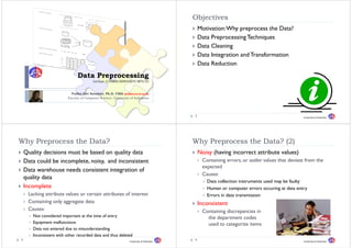
1. Objectives
Obj ti
Motivation: Why preprocess the Data?
Data Preprocessing Techniques
Data Cleaning
Data Integration and Transformation
Data Reduction
Data Preprocessing
Lecture 3/DMBI/IKI83403T/MTI/UI
Yudho Giri Sucahyo, Ph.D, CISA (yudho@cs.ui.ac.id)
y , , (y )
Faculty of Computer Science, University of Indonesia
2 University of Indonesia
Why Preprocess the D t ?
Wh P th Data? Why P
Wh Preprocess the Data? (2)
th D t ?
Quality decisions must be based on quality data Noisy (having incorrect attribute values)
Data could be incomplete, noisy, and inconsistent Containing errors, or outlier values that deviate from the
expected
Data warehouse needs consistent integration of
Causes:
q
quality data
y
Data collection instruments used may be faulty
Incomplete Human or computer errors occuring at data entry
Lacking
L ki attribute values or certain attributes of i
ib l i ib f interest Errors in data transmission
Containing only aggregate data Inconsistent
Causes: Containing discrepancies in
Not considered important at the time of entry the department codes
Equipment malfunctions used to categorize items
Data not entered due to misunderstanding
Inconsistent with other recorded data and thus deleted
3 University of Indonesia
4 University of Indonesia

2. Why P
Wh Preprocess the Data? (3)
th D t ? Data P
D t Preprocessing Techniques
i T h i
“Clean” the data by filling in missing values, smoothing
Clean values Data Cleaning
noisy data, identifying or removing outliers, and resolving To remove noise and correct inconsistencies in the data
inconsistencies.
inconsistencies Data Integration
Some examples of inconsistencies: Merges data from multiple sources into a coherent data
g p
customer_id vs cust_id store, such as a data warehouse or a data cube
Bill vs William vs B.
Data Transformation
Some attributes may be inferred from others. Data Normalization (to improve the accuracy and efficiency of
cleaning including detection and removal of redundancies
g g mining algorithms involving distance measurements E g
E.g.
that may have resulted. Neural networks, nearest-neighbor)
Data Di
D t Discretization
ti ti
Data Reduction
5 University of Indonesia
6 University of Indonesia
Data P
D t Preprocessing Techniques (2)
i T h i Data P
D t Preprocessing Techniques (3)
i T h i
Data Reduction
Warehouse may store terabytes of data
Complex data analysis/mining may take a very long time to run on the
p y g y y g
complete data set
Obtains a reduced representation of the data set that is much smaller in
p
volume, yet produces the same (or almost the same) analytical results.
Strategies for Data Reduction
Data aggregation (e.g., building a data cube)
Dimension reduction (e.g. removing irrelevant attributes through
correlation analysis)
Data compression (e.g. using encoding schemes such as minimum length
encoding or wavelets)
Numerosity reduction
Generalization
7 University of Indonesia
8 University of Indonesia

3. Data Cl
D t Cleaning – Mi i
i Missing Values
V l Data Cl
D t Cleaning – Mi i
i Missing V l
Values (2)
1. Ignore the tuple 5.
5 Use the attribute mean for all samples belonging to the
Usually done when class label is missing classification same class as the given tuple same credit risk
Not effective when the missing values in attributes spread in category
t
different tuples
6. Use the most probable value to fill in the missing value
2. Fill
F ll in the missing value manually: tedious + infeasible?
h l ll d f bl ? Determined with regression, inference-based tools such as
3. Use a global constant to fill in the missing value
g g Bayesian formalism, or decision tree induction
y
‘unknown’, a new class?
Mining program may mistakenly think that they form an Methods 3 to 6 bias the data. The filled-in value may not be
y
interesting concept, since they all have a value in common correct. However, method 6 is a popular strategy, since:
not recommended It uses the most information from the present data to predict missing values
4. Use the attribute mean to fill in the missing value There is a greater chance that the relationships between income and the other
attributes are preserved
preserved.
avg i
income
9 University of Indonesia
10 University of Indonesia
Data Cleaning – Data Cleaning – Noisy Data
Noise
N i and Incorrect (Inconsistent) Data
dI t (I i t t) D t Binning Methods
Bi i M th d
Noise is a random error or variance in a measured variable
variable. * Sorted data for price ( dollars): 4, 8, 9, 15, 21, 21, 24, 26, 25, 28, 29, 34
p (in ) , , , , , , , , , , ,
* Partition into (equidepth) bins of depth 3, each bin contains three values:
How can we smooth out the data to remove the noise?
- Bin 1: 4, 8, 9, 15
, , ,
Binning Method - Bin 2: 21, 21, 24, 26
Smooth a sorted data value by consulting its “neighborhood”, that - Bin 3: 25, 28, 29, 34
, , ,
is, the values around it. * Smoothing by bin means:
The sorted values are distributed into a number of buckets, or bins. - Bin 1: 9, 9, 9, 9
, , ,
Because binning methods consult the neighborhood of values, they - Bin 2: 23, 23, 23, 23
perform local smoothing. - Bin 3: 29, 29, 29, 29
, , ,
Binning is also uses as a discretizatin technique (will be discussed * Smoothing by bin boundaries: the larger the width, the greater the effect
later) - Bin 1: 4, 4, 4, 15
, , ,
- Bin 2: 21, 21, 26, 26
- Bin 3: 25, 25, 25, 34
, , ,
11 University of Indonesia
12 University of Indonesia

4. Data Cleaning – Noisy Data Data Cleaning – Noisy Data
Clustering
Cl t i Regression
R i
Similar values are organized into groups or clusters
groups, clusters. Data can be smoothed by y
Values that fall outside of the set of clusters may be fitting the data to a
considered outliers.
id d tli function,
function such as with Y1
regression.
Linear regression i l
Li i involves Y1’ y=x+1
finding the best line to fit
two variables, so that one
variable can be used to X1 x
predict the other.
Multiple linear regression
p g
> 2 variables,
multidimensional surface
13 University of Indonesia
14 University of Indonesia
Data S
D t Smoothing vs Data Reduction
thi D t R d ti Data Cl
D t Cleaning - I
i Inconsistent Data
i t tD t
Many methods for data smoothing are also methods May be corrected manually
manually.
for data reduction involving discretization. Errors made at data entry may be corrected by
Examples performing a paper trace, coupled with routines designed
f i t l d ith ti d i d
Binning techniques
g q reduce the number of distinct values to help correct the inconsistent use of codes.
per attribute. Useful for decision tree induction which Can also using tools to detect the violation of known
repeatedly make value comparisons on sorted data. data constraints.
Concept hierarchies are also a form of data discretization
that can also be used for data smoothng. g
Mapping real price into inexpensive, moderately_priced,
p
expensive
Reducing the number of data values to be handled by the
mining process.
15 University of Indonesia
16 University of Indonesia

5. Data I t
D t Integration and Transformation
ti dT f ti Data T
D t Transformation
f ti
Data Integration: combines data from multiple data stores Data are transformed into forms appropriate for mining
Schema integration Methods:
integrate metadata from different sources Smoothing: binning, clustering, and regression
Entity identification p
y problem: identify real world entities from
y Aggregation: summarization, data cube construction
gg g
multiple data sources, e.g., A.cust-id ≡ B.cust-# Generalization: low-level or raw data are replaced by higher-
level concepts through the use of concept hierarchies
p g p
Detecting d
D t ti and resolving d t value conflicts
l i data l fli t
Street city or country
for the same real world entity, attribute values from different
Numeric attributes of age young, middle-aged,
young middle-aged senior
sources are different
Normalization: attribute data are scaled so as to fall within a
possible reasons: different representations, different scales (feet small specified range, such as 0.0 to 1.0
range 00 10
vs metre) Useful for classification involving neural networks, or distance
measurements such as nearest neighbor classification and clustering
17 University of Indonesia
18 University of Indonesia
Data T
D t Transformation (2)
f ti Data R d ti
D t Reduction – D t Cube Aggregation
Data C b A ti
Normalization: scaled to f ll within a small, specified range
N li i l d fall i hi ll ifi d Data consist of sales per quarter, for several years. User
quarter years
interested in the annual sales (total per year) data can
min-max normalization
be
b aggregated so that the resulting data summarize the
d h h li d i h
v − minA
v' = (new _ maxA − new _ minA) + new _ minA total sales per year instead of per quarter.
maxA − minA
Resulting data set is smaller in volume, without loss of
z-score normalization information necessary for the analysis task
task.
v − mean A See Figure 3.4 [JH]
v'=
stand _ d
t d dev A
normalization by decimal scaling
y g
v
v' = Where j is the smallest integer such that Max(| v' |)<1
|) 1
10 j
19 University of Indonesia
20 University of Indonesia

6. Dimensionality Reduction
Di i lit R d ti Dimensionality Reduction (2)
Di i lit R d ti
Datasets for analysis may contain hundreds of The goal of attribute subset selection (also known as
attributes, many of which may be irrelevant to the feature selection) is to find a minimum set of attributes such
that the resulting probability distribution of the data classes is
mining t k or redundant.
i i task, d d t
as close as possible to the original distribution obtained using
Leaving out relevant attributes or keeping irrelevant all attributes.
attributes can cause confusion for the mining For d attributes, there are 2d possible subsets.
algorithm, poor quality of discovered patterns. The best (and worst) attributes are typically determined using
Added volume of irrelevant or redundant attributes tests of statistical significance. Attribute evaluation measures
can slow d
l down the mining process.
th i i such as information gain can be used
used.
Heuristic methods
Dimensionality reduction reduces the data set size by
Stepwise f
St i forward selection
d l ti
removing such attributes from it. Stepwise backward selection (or combination of both)
Decision tree induction
21 University of Indonesia
22 University of Indonesia
Dimensionality Reduction (3)
Example of Decision Tree Induction
E l fD i i T I d ti Data C
D t Compression
i
Initial attribute set:
Data encoding or transformations are applied so as to
{A1, A2, A3, A4, A5, A6} obtain a reduced or compressed representation of the
original data
data.
A4 ? Lossless data compression technique: If the original data
can b reconstructed f
be d from the compressed data without
h dd ih
any loss of information.
A1? A6?
Lossy data compression technique: we can reconstruct
only an approximation of the original data.
y pp g
Two popular and effective methods of lossy data
Class 2
Class 1 Class 2 Class 1 compression: wavelet transformts and principal components
analysis.
> Reduced attribute set: {A1, A4, A6}
23 University of Indonesia
24 University of Indonesia

7. Data C
D t Compression (2)
i Numerosity Reduction
N it R d ti
Parametric methods:
Assume the data fits some model, estimate model parameters,
store only the parameters, and discard the data (except
parameters
possible outliers).
Original Data
Oi i lD t Compressed
C d Log-linear models: obtain value at a point in m-D space as the
Data product on appropriate marginal subspaces. (see Slide 14)
lossless
l l Non-parametric
Non parametric methods:
No assume models
Three major families:
Clustering (see Slide 13)
Original Data Histograms
Approximated Sampling
25 University of Indonesia
26 University of Indonesia
Numerosity Reduction - Hi t
N it R d ti Histograms Numerosity Reduction - S
N it R d ti Sampling
li
A popular d reduction
l data d i
40 Allows a large data set to be represented by a much
technique 35 smaller random sample (or subset) of the data.
Divide data into buckets Choose a representative subset of th data
Ch t ti b t f the d t
30
and store average (sum) for Simple random sampling may have very poor performance in
each b k
h bucket 25 the
th presence of skew
f k
Partitionng rules: 20 Develop adaptive sampling methods
Equiwidth Stratified sampling:
15
Approximate the percentage of each class (or subpopulation of
Equidepth
10 interest) in the overall database
) h ll d b
Etc. Used in conjunction with skewed data
5
Simple
Si l random sample without replacement (SRSWOR)
d l ih l
0 Simple random sample with replacement (SRSWR)
10000 30000 50000 70000 90000
27 University of Indonesia
28 University of Indonesia

8. Numerosity Reduction – S
N it R d ti Sampling (2)
li Numerosity Reduction – S
N it R d ti Sampling (3)
li
Raw Data Cluster/Stratified Sample
Raw Data
29 University of Indonesia
30 University of Indonesia
Discretization and concept hierarchy
Discretization and Concept Hierarchy
Di ti ti dC t Hi h generation for numeric d t
ti f i data
Discretization can be used to reduce the number of Binning
values for a given continuous attribute, by dividing the Histogram analysis
range of the attribute into intervals. I t
f th tt ib t i t i t l Interval l b l
l labels Clustering analysis
can then be used to replace actual data values. Entropy-based discretization
py
Concept hierarchies can be used to reduce the data Segmentation by natural partitioning 3-4-5 rule
by collecting and replacing low level concepts (such as
numeric values for the attribute age) by higher level
concepts (such as young, middle-aged, or senior).
young middle aged senior)
31 University of Indonesia
32 University of Indonesia

9. Concept hierarchy generation for
Example of 3-4-5 rule
E l f34 5 l categorical data
t i ld t
count
Categorical data are discrete data. Have a finite
data
number of distinct values, with no ordering among the
Step -$351 -$159 profit $1,838 $4,700 values. Ex Location
values Ex. Location, job category.
category
1:
Specification of a set of attributes:
Min Low (i.e, 5%-tile) High(i.e, 95%-0 tile) Max
Step 2: msd=1,000 Low=-$1,000 High=$2,000
(-$1,000 - $2,000)
Step 3:
Concept hierarchy can be country
(-$1,000 - 0) (0 -$ ($1,000 - $2,000) 15 distinct values
1,000) automatically generated
Step
(-$4000 -$5,000)
based on the number of province_or_ state
4:
($2,000 - $5, 000)
distinct values per attribute 65 distinct values
($1,000 $2,
($1 000 - $2 000)
in the given attribute set.
(-$400
( $400 - 0) (0 - $1 000)
$1,000)
(0 -
($1,000
(-$400 - - ($2,000 -
The attribute with the most city 3567 distinct values
-$300) $200)
($200 - $1,200) $3,000)
distinct l
di ti t values is placed at
i l d t
(
($1,200 -
$400)
(-$300 - $1,400)
($3,000 -
-$200)
(-$200 -
($400 -
$600)
($1,400 -
$1,600)
$4,000)
($4,000
the lowest level of the street 674,339 distinct values
-$100) ($600 -
$800) ($800 -
($1,600
($1 600 -
$1,800)
($1,800 -
-
$5,000) hierarchy.
hierarchy
(-$100 - $1,000) $2,000)
33 0)
University of Indonesia
34 University of Indonesia
Conclusion
C l i References
R f
Data preparation is a big issue for both warehousing [JH] Jiawei Han and Micheline Kamber, Data Mining:
Kamber
and mining Concepts and Techniques, Morgan Kaufmann, 2001.
Data preparation includes
Data cleaningg
Data integration and Data transformation
Data reduction and feature selection
Discretization
A lot a methods have been d l
l t th d h b developed but still an
d b t till
active area of research
35 University of Indonesia
36 University of Indonesia