1. TRANSPORTATION PROBLEM
Transportation problem is one of the subclasses of LPP’s in which the objective is to
transport various quantities of a single homogeneous commodity, that are initially stored at
various origins to different destinations in such a way that the total transportation cost is
minimum. To achieve this objective we must know the amount and location of available
supplies and the quantities demanded. In addition, we must know the costs that result from
transporting one unit of commodity from various origins to various destinations.
Mathematical Formulation of the Transportation Problem
A transportation problem can be stated mathematically as a Linear Programming Problem as
below:
Minimize Z =
subject to the constraints
= ai , i = 1, 2,…..,m
= bj , j = 1, 2,…..,m
xij ≥ 0 for all i and j
Where, ai = quantity of commodity available at origin i
bj= quantity of commodity demanded at destination j
cij= cost of transporting one unit of commodity from ith origin to jth
destination
xij = quantity transported from ith origin to jth destination
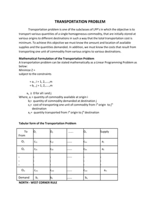
Tabular form of the Transportation Problem
To D1 D2 ……. Dn Supply
From
O1 c11 c12 ……. c1n a1
O2 c21 c22 ……. c2n a2
. . . ……. . .
. . . . .
. . . . .
Om cm1 cm2 ……. cmn am
Demand b1 b2 ……. bn
NORTH - WEST CORNER RULE

2. Step1:Identify the cell at North-West corner of the transportation matrix.
Step2:Allocate as many units as possible to that cell without exceeding supply or
demand; then cross out the row or column that is exhausted by this assignment
Step3:Reduce the amount of corresponding supply or demand which is more by allocated
amount.
Step4:Again identify the North-West corner cell of reduced transportation matrix.
Step5:Repeat Step2 and Step3 until all the rim requirements are satisfied.
Vogel’s Approximation Method (VAM)
Step-I: Compute the penalty values for each row and each column. The penalty will be
equal to the difference between the two smallest shipping costs in the row or column.
Step-II: Identify the row or column with the largest penalty. Find the first basic variable which
has the smallest shipping cost in that row or column. Then assign the highest
possible value to that variable, and cross-out the row or column which is
exhausted.
Step-III: Compute new penalties and repeat the same procedure until all the rim
requirements are satisfied.
An example for Vogel’s Method
Find the IBFS of the following transportation problem by using Penalty Method.
D1 D2 D3
Supply
10
6 7 8
15
15 80 78
15 5 5
Step 1: Compute the penalties in each row and each column .
Supply Row Penalty
10 7-6=1
6 7 8
Supply 15 78-15=63
Row Penalty
15 80 78
Demand 15 5 5 10 7-6=1
Step 2: Identify the largest penalty and choose least cost cell to corresponding this penalty
6 7 8
Column Penalty 15-6=9 80-7=73 78-8=70
15 78-15=63
15 80 78
Demand 15 5 5
Column Penalty 15-6=9 80-7=73 78-8=70

3. Step-3: Allocate the amount 5 which is minimum of corresponding row supply and column
demand and then cross out column2
Supply Row Penalty
5
10 7-6=1
6 7 8
15 78-15=63
15 80 78
Demand 15 5 5
Column Penalty 15-6=9 80-7=73 78-8=70
Step-4: Recalculate the penalties
Supply Row Penalty
5
5 8-6=2
6 7 8
15 78-15=63
15 80 78
Demand 15 X 5
Column Penalty 15-6=9 78-8=70
Supply Row Penalty
5
5 8-6=2
Step-5: Identify the6largest penalty and choose least cost cell to corresponding this penalty
7 8
15 78-15=63
15 80 78
Demand 15 X 5
Column Penalty 15-6=9 78-8=70

4. Step-6: Allocate the amount 5 which is minimum of corresponding row supply and column
demand, then cross out column3
Supply Row Penalty
5 5
5 8-6=2
6 7 8
15 78-15=63
15 80 78
Demand 15 X X
Column Penalty 15-6=9
Step-7: Finally allocate the values 0 and 15 to corresponding cells and cross out column 1
D1 D2 D3 Supply
0 5 5
X
O1 6 7 8
15
X
O2 15 80 78
Demand X X X
Solution of the problem
Now the Initial Basic Feasible Solution of the transportation problem is
X11=0, X12=5, X13=5, and X21=15 and
Total transportation cost = (0x6)+(5x7)+(5x8)+(15x15)
= 0+35+40+225
= 300.