

Recomendados
Recomendados
Más contenido relacionado
La actualidad más candente
La actualidad más candente (20)
Destacado
Destacado (20)
Similar a kenpave
Similar a kenpave (20)
Último
Último (20)
kenpave
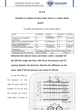
- 1. UNIVERSIDAD PERUANA LOS ANDES CARRERA PROFESIONAL INGENIERIA CIVIL SOLANORAMOS JAVIER JHEFERSON (X-C1) CE 475 Example on analysis of stress-strain state in a 5-layer elastic system Consider the pavement cross-section given: Layer Thickness Elastic modulus Poisson’s Ratio Density Surface Course (Asphalt Concrete Mixture) 4” 350,000 psi .2 155 pcf Base Course (Asphalt Treated Base, Emulsified Asphalt Mixture) 6” 150,000 psi .3 150 pcf Aggregate Subbase 6” 85,000 psi .4 100 pcf Crushed Aggregate Subbase (Rockcap) 12” 120,000 psi .4 90 pcf Geotextile Fabric For layer separation. No structural support value Subgrade (Soft clay material) N/A 5,000 psi .45 90 pcf Determine the state of stress and strains under a standard 18- kip (80-kN) single axle load, with 85 psi tire pressure and 13” spacing between the dual tires. Examine the difference on the stress state if the tire pressure was raised to 120 psi. To see the effect of tire pressure on the state of stress, solve the problem for 85 psi, and find stresses and strains under point 1 (center of
- 2. UNIVERSIDAD PERUANA LOS ANDES CARRERA PROFESIONAL INGENIERIA CIVIL SOLANORAMOS JAVIER JHEFERSON (X-C1) one tire) at all depths as shown. Note that same values will be obtained at point 4 because of similarity. Plot results of stresses and strains under point 1 at all depths, and see the difference. Note KENPAVE shows positive values for “compressive” and “negative values for “tensile”, since the +z axis is in the downward direction. SOLUCION - DETERMINE EL ESTADO DE ESFUERZO DE LA ESTRUCTURA MOSTRADA. Además la estructura anterior está sometida a una carga standard de un eje simple de 18-kips (18,000 lbs o 80-kN) con
- 3. UNIVERSIDAD PERUANA LOS ANDES CARRERA PROFESIONAL INGENIERIA CIVIL SOLANORAMOS JAVIER JHEFERSON (X-C1) presión en las llantas de 85 psi y separación entre las llantas de 13”. Examine la diferencia de estado de esfuerzo con presión en las llantas de 120 psi. Además de calcular los esfuerzos en el centro de una llanta, calcular los mismos en las siguientes ubicaciones. 1. SOLUCION ELASTICA MULTICAPA: 1. INGRESO A PANTALLA PRINCIPAL.- Digitar el nombre del archivo "ASFALTO" en el casillero Filename, seguidamente hacer click en la opción LAYERINP para ingresar al menú principal del KENPAVE.
- 4. UNIVERSIDAD PERUANA LOS ANDES CARRERA PROFESIONAL INGENIERIA CIVIL SOLANORAMOS JAVIER JHEFERSON (X-C1) 2. Ingresaremos al menú principal del programa: Se tiene que ir de izquierda a derecha llenando los datos según se indica. Si está en rojo (ej. input) se tiene que hacer click en el icono respectivo y llenar la información. Si está en azul (ej. default) son valores predeterminados, se pueden dejar ahí o cambiarse si se desea.
- 5. UNIVERSIDAD PERUANA LOS ANDES CARRERA PROFESIONAL INGENIERIA CIVIL SOLANORAMOS JAVIER JHEFERSON (X-C1) 3. DEFINICION DE NUEVO PROYECTO.- En el menú File hacer click y seleccionar la opción New para insertar un nuevo proyecto. 4. DEFINICIÓN DE LAS CARACTERÍSTICAS DEL SISTEMA.- Definir las características del sistema a analizar abriendo el menú. General, donde se abrirá la ventana General Information of LAYERINP for Set No.1, como podemos apreciar en la figura. En la casilla TITLE se escribirá el título del proyecto.
- 6. UNIVERSIDAD PERUANA LOS ANDES CARRERA PROFESIONAL INGENIERIA CIVIL SOLANORAMOS JAVIER JHEFERSON (X-C1) Para este caso ingresaremos en el casillero Number of layers (número de capas), 5 y en el casillero Number of Z coordinates for análisis (número de coordenadas en el eje Z a analizar), 5 ya que analizaremos en 5 profundidades distintas, además sobre el casillero System of unites colocamos el valor de 0 ya que trabajaremos en unidades inglesas. Finalmente presionamos OK. 5. UBICACIÓN DE LAS PROFUNDIDAES A ANALIZAR.- Hacemos click en el menú Zcood de donde aparecerá la ventana Zcoordinates of Response for Data Set No. 1, en el cual insertaremos la ubicación de las profundidades a analizar. 5
- 7. UNIVERSIDAD PERUANA LOS ANDES CARRERA PROFESIONAL INGENIERIA CIVIL SOLANORAMOS JAVIER JHEFERSON (X-C1) Para ello insertamos la profundidad de cada punto a analizar tomando como inicio la superficie del pavimento, en este caso se ha insertado la ubicación de las 5 profundidades dadas en el ejemplo. 6. INGRESO COEFICIENTE DE POISSON DE LAS CAPAS.- Ingresamos al menú Layer en el cual insertaremos los valores de los módulos de Poisson para cada capa, en la ventana Layer Thickness, Poisson of each period for Data Set No. 1
- 8. UNIVERSIDAD PERUANA LOS ANDES CARRERA PROFESIONAL INGENIERIA CIVIL SOLANORAMOS JAVIER JHEFERSON (X-C1) 7. INGRESO DEL MODULO DE ELASTICIDAD DE LAS CAPAS.- Ingresamos al menú Moduli en el cual insertaremos los valores de los módulos de elasticidad para capa, automáticamente aparece la ventana Layer Modulus of each period for Data Set No. 1; para continuar hacemos clic en el botón Period1.
- 9. UNIVERSIDAD PERUANA LOS ANDES CARRERA PROFESIONAL INGENIERIA CIVIL SOLANORAMOS JAVIER JHEFERSON (X-C1) 8. INGRESO DE LAS CARGAS Y LOS PUNTOS DE ANALISIS.- Ingresamos al menú Load, seguidamente aparecerá la ventana
- 10. UNIVERSIDAD PERUANA LOS ANDES CARRERA PROFESIONAL INGENIERIA CIVIL SOLANORAMOS JAVIER JHEFERSON (X-C1) Load Information for Data Set No. 1. Para rellenar este cuadro mostramos la figura que facilitara la comprensión de los valores: 9. En el casillero LOAD se colocara el valor de 0; 1 o 2 depende del tipo de sistema de carga sea, en este caso ingresaremos el valor de 1 ya que este es un sistema dual simple.
- 11. UNIVERSIDAD PERUANA LOS ANDES CARRERA PROFESIONAL INGENIERIA CIVIL SOLANORAMOS JAVIER JHEFERSON (X-C1) A CONTINUACION INGRESAMOS LOS PUNTOS DE ANALISIS Hacemos doble clic en el valor del casillero LOAD, de inmediato aparecerá la ventana mostrada en la cual ingresamos los puntos de análisis en la dirección YPT.
- 12. UNIVERSIDAD PERUANA LOS ANDES CARRERA PROFESIONAL INGENIERIA CIVIL SOLANORAMOS JAVIER JHEFERSON (X-C1) 10. Finalmente hacemos clic en OK hasta llegar al menú principal. Guardamos el archivo haciendo clic en Save As y luego para salir del menú presionamos Exit. 2. ANALISIS Y VISUALIZACION DE RESULTADOS: Guardado el archivo, volvemos a la ventana principal del KENPAVE donde presionamos el botón KENLAYER para procesar los datos.
- 13. UNIVERSIDAD PERUANA LOS ANDES CARRERA PROFESIONAL INGENIERIA CIVIL SOLANORAMOS JAVIER JHEFERSON (X-C1) De inmediato aparecerá el siguiente mensaje, el cual nos muestra en que la ubicación en donde se guardaron los resultados en formato TXT (subrayado). VISUALIZACION DE RESULTADOS.- Para visualizar los resultados hacemos clic en LGRAPH, el programa arrojara la representación gráfica del sistema analizado. De igual manera podemos imprimir esta hoja, de lo contrario solamente abrimos el archivo C: /ASFALTO.TXT ASFALTO ASFALTO.DAT
- 14. UNIVERSIDAD PERUANA LOS ANDES CARRERA PROFESIONAL INGENIERIA CIVIL SOLANORAMOS JAVIER JHEFERSON (X-C1) 3. KENPAVE OUTPUT AS TEXT (RENDIMIENTO) INPUT FILE NAME -C:ASFALTO.DAT NUMBER OF PROBLEMS TO BE SOLVED = 1 TITLE -Class Example for 5-layer Analysis under 85 psi tire pressure MATL = 1 FOR LINEAR ELASTIC LAYERED SYSTEM NDAMA = 0, SO DAMAGE ANALYSIS WILL NOT BE PERFORMED NUMBER OF PERIODS PER YEAR (NPY) = 1 NUMBER OF LOAD GROUPS (NLG) = 1 TOLERANCE FOR INTEGRATION (DEL) -- = 0.001 NUMBER OF LAYERS (NL)------------- = 5
- 15. UNIVERSIDAD PERUANA LOS ANDES CARRERA PROFESIONAL INGENIERIA CIVIL SOLANORAMOS JAVIER JHEFERSON (X-C1) NUMBER OF Z COORDINATES (NZ)------ = 14 LIMIT OF INTEGRATION CYCLES (ICL)- = 80 COMPUTING CODE (NSTD)------------- = 9 SYSTEM OF UNITS (NUNIT)------------= 0 Length and displacement in in., stress and modulus in psi unit weight in pcf, and temperature in F THICKNESSES OF LAYERS (TH) ARE : 4 6 6 12 POISSON'S RATIOS OF LAYERS (PR) ARE : 0.2 0.3 0.4 0.4 0.45 VERTICAL COORDINATES OF POINTS (ZC) ARE: 0 4 10 16 28 ALL INTERFACES ARE FULLY BONDED FOR PERIOD NO. 1 LAYER NO. AND MODULUS ARE : 1 3.500E+05 2 1.500E+05 3 8.500E+04 4 1.200E+05 5 5.000E+03 LOAD GROUP NO. 1 HAS 2 CONTACT AREAS CONTACT RADIUS (CR)--------------- = 4.11 CONTACT PRESSURE (CP)------------- = 85 NO. OF POINTS AT WHICH RESULTS ARE DESIRED (NPT)-- = 5 WHEEL SPACING ALONG X-AXIS (XW)------------------- = 0 WHEEL SPACING ALONG Y-AXIS (YW)------------------- = 13 RESPONSE PT. NO. AND (XPT, YPT) ARE: 1 0.000 0.000 2 0.000 6.500
- 16. UNIVERSIDAD PERUANA LOS ANDES CARRERA PROFESIONAL INGENIERIA CIVIL SOLANORAMOS JAVIER JHEFERSON (X-C1) 3 0.000 4.110 4 0.000 13.000 5 0.000 8.890 PERIOD NO. 1 LOAD GROUP NO. 1 4. EXAMPLE ON 5 LAYER SYSTEM SUBJECTED TO 18-KIP ESAL, WITH 85 & 120 PSI TIRE PRESSURE FOR POINT 1 UNDER CENTER OF ONE TIRE (X=0, Y=0) Vertical Deflection Vertical Stress Major P. Stress Minor P. Stress Intermediat e P. Stress Vertical Strain Major P. Strain Minor P. Strain Horizont al P. Strain q z Dz sz s1 s3 s2 ez e1 e3 et 0 0.01518 85 118.491 114.998 116.144 1.94E-04 2.07E-04 1.95E-04 1.99E-04 4 0.01422 46.181 46.282 -17.949 -13.606 1.50E-04 1.50E-04 -7.00E-05 -7.00E-05 10 0.01316 14.516 14.847 -7.704 -4.482 1.21E-04 1.23E-04 -7.21E-05 -7.21E-05 16 0.01249 6.886 7.623 0.012 0.044 7.73E-05 8.94E-05 -3.59E-05 -3.54E-05 28 0.01172 0.856 0.857 -11.863 -11.051 8.35E-05 8.35E-05 -6.49E-05 -6.49E-05 0 0.0165 120 160.684 152.869 155.309 2.83E-04 2.83E-04 2.56E-04 2.56E-04 4 0.01524 56.4 56.484 -26.12 -21.543 1.88E-04 1.89E-04 -9.46E-05 -9.46E-05 10 0.014 15.864 16.201 -8.619 -5.121 1.33E-04 1.36E-04 -7.96E-05 -7.96E-05 16 0.01327 7.396 8.18 0.034 0.055 8.29E-05 9.58E-05 -3.84E-05 -3.80E-05 28 0.01245 0.905 0.906 -12.561 -11.69 8.84E-05 8.84E-05 -6.87E-05 -6.87E-05 Point 1 at x=0, y=0 85psi120psi
- 17. UNIVERSIDAD PERUANA LOS ANDES CARRERA PROFESIONAL INGENIERIA CIVIL SOLANORAMOS JAVIER JHEFERSON (X-C1) Tire Pressure Depth Vertical Deflection Vertical Stress Major P. Stress Minor P. Stress Intermediate P. Stress Vertical Strain Major P. Strain Minor P. Strain Horizontal P. Strain z Dz sz s1 s3 s2 ez e1 e3 et 85 PSI 0 Surface 0.01511 -85.0 -118.5 -115.0 -116.1 -1.9E-04 -2.1E-04 -1.9E-04 -2.0E-04 85 4 Bottom of AC Surface 0.01415 -46.2 -46.3 17.9 13.6 -1.5E-04 -1.5E-04 7.0E-05 7.0E-05 85 10 Bottom of ATB layer 0.0131 -14.5 -14.8 7.7 4.5 -1.2E-04 -1.2E-04 7.2E-05 7.2E-05 85 16 Top of Subgrade 0.01243 -6.9 -7.6 0.0 0.0 -7.7E-05 -8.9E-05 3.6E-05 3.5E-05 85 28 Below subgrade surface by 1/2 pavement depth 0.01166 -0.9 -0.9 11.9 11.1 -8.4E-05 -8.4E-05 6.5E-05 6.5E-05 120 PSI 0 Surface 0.0165 -120.0 -160.7 -152.9 -155.3 -2.8E-04 -2.8E-04 -2.6E-04 -2.6E-04 120 4 Bottom of AC Surface 0.01524 -56.4 -56.5 26.1 21.5 -1.9E-04 -1.9E-04 9.5E-05 9.5E-05 120 10 Bottom of ATB layer 0.014 -15.9 -16.2 8.6 5.1 -1.3E-04 -1.4E-04 8.0E-05 8.0E-05 120 16 Top of Subgrade 0.01327 -7.4 -8.2 0.0 -0.1 -8.3E-05 -9.6E-05 3.8E-05 3.8E-05 120 28 Below subgrade surface by 1/2 pavement depth 0.01245 -0.9 -0.9 12.6 11.7 -8.8E-05 -8.8E-05 6.9E-05 6.9E-05 Depth Vertical Deflection Vertical Stress Major P. Stress Minor P. Stress Intermediate P. Stress Vertical Strain Major P. Strain Minor P. Strain Horizontal P. Strain q z Dz sz s1 s3 s2 ez e1 e3 et Note: Stresses and strains are reversed to show - for compresssion and + for tenstion Note: Stresses and strains here are as obtained from Kenpave (+ for compression and - for tenstion) Depth Vertical Deflection Vertical Stress Major P. Stress Minor P. Stress Intermediate P. Stress Vertical Strain Major P. Strain Minor P. Strain Horizontal P. Strain q z Dz sz s1 s3 s2 ez e1 e3 et 0 Surface 0.01511 85.0 118.5 115.0 116.1 1.9E-04 2.1E-04 1.9E-04 2.0E-04 4 Bottom of AC Surface 0.01415 46.2 46.3 -17.9 -13.6 1.5E-04 1.5E-04 -7.0E-05 -7.0E-05 10 Bottom of ATB layer 0.0131 14.5 14.8 -7.7 -4.5 1.2E-04 1.2E-04 -7.2E-05 -7.2E-05 16 Top third of CAB 0.01243 6.9 7.6 0.0 0.0 7.7E-05 8.9E-05 -3.6E-05 -3.5E-05 28 Below subgrade surface by 1/2 pavement depth 0.01166 0.9 0.9 -11.9 -11.1 8.4E-05 8.4E-05 -6.5E-05 -6.5E-05 0 Surface 0.0165 120.0 160.7 152.9 155.3 2.8E-04 2.8E-04 2.6E-04 2.6E-04 4 Bottom of AC Surface 0.01524 56.4 56.5 -26.1 -21.5 1.9E-04 1.9E-04 -9.5E-05 -9.5E-05 10 Bottom of ATB layer 0.014 15.9 16.2 -8.6 -5.1 1.3E-04 1.4E-04 -8.0E-05 -8.0E-05 16 Top third of CAB 0.01327 7.4 8.2 0.0 0.1 8.3E-05 9.6E-05 -3.8E-05 -3.8E-05 28 Below subgrade surface by 1/2 pavement depth 0.01245 0.9 0.9 -12.6 -11.7 8.8E-05 8.8E-05 -6.9E-05 -6.9E-05 Note: Stresses and strains here are as obtained from Kenpave (+ for compression and - for tenstion) 85psi
- 18. UNIVERSIDAD PERUANA LOS ANDES CARRERA PROFESIONAL INGENIERIA CIVIL SOLANORAMOS JAVIER JHEFERSON (X-C1) 0 5 10 15 20 25 30 0.01 0.011 0.012 0.013 0.014 0.015 0.016 Depthz,in Deflection Value Deflection Variation with Depth at Point 1 85 PSI 120 PSI 0 5 10 15 20 25 30 -180.0 -150.0 -120.0 -90.0 -60.0 -30.0 0.0 Depth,z,in Vertical Stress,Sigma z, psi Vertical Stress Variation with Depth at Point 1 85 PSI 120 PSI
- 19. UNIVERSIDAD PERUANA LOS ANDES CARRERA PROFESIONAL INGENIERIA CIVIL SOLANORAMOS JAVIER JHEFERSON (X-C1) 0 5 10 15 20 25 30 -3.0E-04 -2.0E-04 -1.0E-04 0.0E+00 Depthz,in Vertical strain, strain z Vertical Strain Variation with Depth at Point 1 85 PSI 120 PSI 0 5 10 15 20 25 30 -3.0E-04 -2.0E-04 -1.0E-04 0.0E+00 1.0E-04 Depthz,in Horizontal strain, strain H Horizontal Strain Variation with Depth at Point 1 85 PSI 120 PSI
- 20. UNIVERSIDAD PERUANA LOS ANDES CARRERA PROFESIONAL INGENIERIA CIVIL SOLANORAMOS JAVIER JHEFERSON (X-C1)