
Recommended
More Related Content
What's hot
What's hot (20)
Similar to Lab 1 kirchhoff’s voltage and current law by kehali bekele haileselassie
Similar to Lab 1 kirchhoff’s voltage and current law by kehali bekele haileselassie (20)
More from kehali Haileselassie
More from kehali Haileselassie (7)
Recently uploaded
Recently uploaded (20)
Lab 1 kirchhoff’s voltage and current law by kehali bekele haileselassie
- 1. Kirchhoff’s Voltage and Current Law Laboratory - #1 Kehali B. Haileselassie& Faisal Abdulrazaqalsaa 07/16/2013 ELC ENG 305 – Circuit Analysis II Instructor - EbrahimForati
- 2. Introduction The purpose of this report is to verify Kirchhoff’s Current Law and Kirchhoff’s Voltage Law by constructing a simple three loop circuit that containing six resistors. The purpose of the report also includes measuring the current through each resistors and the voltage at each nodes in the circuit. The circuit was built using a given Elenco DC power supply (Model XP-770), digital multi-meter, breadboard, electrical wires and six random resistors. Kirchhoff’s Current Law (KCL) and Kirchhoff’s Voltage Law (KVL) is very important to analysis a linear circuit. It is mainly deals to relate voltage to current and resistance. Kirchhoff’s Voltage Law (KVL) states that the algebraic sum of all voltages in a closed loop must be equal to zero. A closed loop is a path in a circuit that does give a return path for a current. Kirchhoff’s Current Law (KCL) deals with the current flowing into and out of a single node. It states that the sum of the current flowing into the node and the current flowing out from the node must equal to zero.
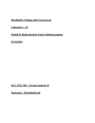
- 3. Procedure The six resistors were chosen randomly from the kit. Their resistance nominal and measured Values of each resistor are shown in the table below. Item Reference Nominal Value (kῼ) Measured Value(kῼ) 1 R1 1 0.98 2 R2 2 1.96 3 R3 2 1.96 4 R4 1 0.98 5 R5 2 1.96 6 R6 1 0.98 Table_1 Data and Analysis We used loop analysis to figure out the voltage of each nodes and the current that flow through each resistors. In addition to Kirchhoff’s law, We applied the ohm’s law ( V = IR ) and mesh’s law to solve the current that passes through each resistors. We measured the voltage across each resistor and the power supply by connecting a voltmeter in parallel with the resistors and the power supply. The simple resistive circuit that we designed to verify KVL and KCL with three loops and tworesistor per loop; three nodes with three branches in this laboratory is shown below in figure 1.
- 4. Figure:1 KVL was applied to the three closed loops of the circuit using the symbolic label stated as in figure 2. The equation is shown below. V4 + V1 - Vs = 0 → -10 + 1KI1 + 1K ( I1 – I2 ) = 0 V5 + V2 – V1 = 0 → 1K ( I2 – I1 ) + 2KI2 + 2K ( I2 – I3 ) = 0 V6 + V3 – V2 = 0 → 2K ( I3 – I2 ) + 1KI3 + 2 I3 = 0 Each node also generates KCL equation. The equation is stated as bellow. ((N2 – N1) 1k)) + ( N2 1k ) + ((N2 – N3 ) 2k) = 0 ((N3– N2) 1k)) + ( N3 2k ) + ((N3 – N4 ) 1k) = 0 ((N4– N3) 1k)) + ( N4 2k ) = 0
- 5. The experimental and analytical measured values of the current and voltage are specified in detail in table 2 and 3. Current Lable Experimental Current (mA) Analytical Current (mA) IS 5.65 5.67568 IR_1 4.23 4.32433 IR_2 0.80 0.810809 IR_3 0.53 0.540541 IR_4 5.65 5.67568 IR_5 1.3 1.35135 IR_6 0.53 0.540541 Table_2 Voltage Label Experimental Voltage ( Volt ) Analytical Voltage ( Volt ) Vs 10.01 10.0 Node Voltage_1 (N1) 10.01 10.0 Node Voltage_2 (N2) 4.402 4.32432 Node Voltage_3 (N3) 1.6504 1.62162 Node Voltage_4 (N4) 1.098 1.08108 VR_1 4.402 4.32432 VR_2 1.6504 1.62162 VR_3 1.098 1.08108 VR_4 5.6521 5.67568 VR_5 2.7516 2.7027 VR_6 0.5524 0.54054 Table_3
- 6. In order to verify the Kirchhoff’s Voltage Law and Kirchhoff’s Current Law, let’s see the algebraic sum of the voltages in each loop and the algebraic sum of the current that flowing into and out of each nodes. Substituted in experimental Voltage: ∑Vloop_1 = V4 + V1 - Vs↔ 5.6521 + 4.402 – 10.01 = 0.0441 ∑Vloop_2 = V5 + V2 – V1↔ 2.7516 + 1.6504 – 4.402 = 0 ∑Vloop_3 = V6 + V3 – V2 ↔ 0.5524 + 1.098 – 1.6504 = 0 ∑ IN_2= IR_4 - IR_1 – IR_5 ↔ 5.65 – 4.3 – 1.3 = 0.05 ∑ IN_3 = IR_5 - IR_2 – IR_6 ↔ 1.3 – 0.80 – 0.53 = -0.03 Substituted in Analytical Voltage and Current: ∑Vloop_1 = V4 + V1 - Vs ↔ 5.67568 + 4.32432 – 10 = 0 ∑Vloop_2 = V5 + V2 – V1 ↔ 2.7027 + 1.62162 – 4.32432 = 0 ∑Vloop_3 = V6 + V3 – V2 ↔ 0.54054 + 1.08108 – 1.62162 = 0 ∑ IN_2= IR_4 - IR_1 – IR_5 ↔ 5.67568 – 4.32433 – 1.35135 = 0 ∑ IN_3 = IR_5 - IR_2 – IR_6 ↔ 1.35135 – 0.810809 – 0.540541 = 0 There was no any error in our calculation because the expected value was zero. But there was still some error between the measured (experimental) values and the calculated (analytical) values. %error = |((measured – calculated) measured)| * 100% To verify the ohm’s law, let’s see a sample calculation below: %error = |((measured – calculated) measured)| * 100% = |((10.01 – 10 ) 10.01)| * 100% = 0.099% %error = |((measured – calculated) measured)| * 100% = |((4.402 – 4.32432)/4.402)| * 100% = 1.764%
- 7. Conclussion Ohm’s law and Kirchhoff’s law are the most basic techniques to analysis linear circuits. The main purpose of this lab was to verify these two laws. There were six unknown current and voltage in the circuit. We did build the circuit in breadboard. In order to verify the accuracy of the values we measured experimentally, we simulated the circuit through using LTspice. We did also calculated analytically by using Kirchhoff’s law and Ohm’s law to predict our calculated value and the experimental values are the same. In addition to that, we applied the percent error analysis as well. The percent error between the experimental values and calculated values are less than three percent. The calculated values, the experimental values and the simulated values from the LTspice are almost the same. As a result, we concluded that the Kirchhoff’s Law (KVL & KCL) and the Ohm’s Law are valid.