More Related Content
Similar to Bresenham derivation
Similar to Bresenham derivation (20)
Bresenham derivation
- 1. Appendix: Derivation of Bresenham’s line algorithm
© E Claridge, School of Computer Science, The University of Birmingham
DERIVATION OF THE BRESENHAM’S LINE ALGORITHM
Assumptions:
● input: line endpoints at (X1,Y1) and (X2, Y2)
● X1 < X2
● line slope ≤ 45o
, i.e. 0 < m ≤ 1
● x coordinate is incremented in steps of 1, y coordinate is computed
● generic line equation: y = mx + b
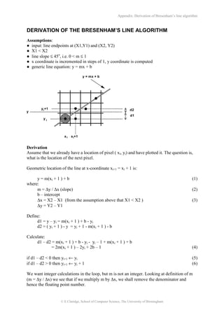
x x +1i i
y i
y +1i
y = mx + b
y
d1
d2
Derivation
Assume that we already have a location of pixel ( xi, yi) and have plotted it. The question is,
what is the location of the next pixel.
Geometric location of the line at x-coordinate xi+1 = xi + 1 is:
y = m(xi + 1 ) + b (1)
where:
m = ∆y / ∆x (slope) (2)
b – intercept
∆x = X2 – X1 (from the assumption above that X1 < X2 ) (3)
∆y = Y2 – Y1
Define:
d1 = y – yi = m(xi + 1 ) + b - yi
d2 = ( yi + 1 ) - y = yi + 1 - m(xi + 1 ) - b
Calculate:
d1 – d2 = m(xi + 1 ) + b - yi - yi – 1 + m(xi + 1 ) + b
= 2m(xi + 1 ) – 2yi + 2b – 1 (4)
if d1 – d2 < 0 then yi+1 ← yi (5)
if d1 – d2 > 0 then yi+1 ← yi + 1 (6)
We want integer calculations in the loop, but m is not an integer. Looking at definition of m
(m = ∆y / ∆x) we see that if we multiply m by ∆x, we shall remove the denominator and
hence the floating point number.
- 2. Appendix: Derivation of Bresenham’s line algorithm
© E Claridge, School of Computer Science, The University of Birmingham
For this purpose, let us multiply the difference ( d1 - d2 ) by ∆x and call it pi:
pi = ∆x( d1 – d2)
The sign of pi is the same as the sign of d1 – d2, because of the assumption (3).
Expand pi:
pi = ∆x( d1 – d2)
= ∆x[ 2m(xi + 1 ) – 2yi + 2b – 1 ] from (4)
= ∆x[ 2 ⋅ (∆y / ∆x ) ⋅ (xi + 1 ) – 2yi + 2b – 1 ] from (2)
= 2⋅∆y⋅ (xi + 1 ) – 2⋅∆x⋅yi + 2⋅∆x⋅b – ∆x result of multiplication by ∆x
= 2⋅∆y⋅xi + 2⋅∆y – 2⋅∆x⋅yi + 2⋅∆x⋅b – ∆x
= 2⋅∆y⋅xi– 2⋅∆x⋅yi + 2⋅∆y + 2⋅∆x⋅b – ∆x (7)
Note that the underlined part is constant (it does not change during iteration), we call it c, i.e.
c = 2⋅∆y + 2⋅∆x⋅b – ∆x
Hence we can write an expression for pi as:
pi = 2⋅∆y⋅xi– 2⋅∆x⋅yi + c (8)
Because the sign of pi is the same as the sign of d1 – d2, we could use it inside the loop to
decide whether to select pixel at (xi + 1, yi ) or at (xi + 1, yi +1). Note that the loop will only
include integer arithmetic. There are now 6 multiplications, two additions and one selection in
each turn of the loop.
However, we can do better than this, by defining pi recursively.
pi+1 = 2⋅∆y⋅xi+1– 2⋅∆x⋅yi+1 + c from (8)
pi+1 – pi = 2⋅∆y⋅xi+1– 2⋅∆x⋅yi+1 + c
- (2⋅∆y⋅xi – 2⋅∆x⋅yi + c )
= 2∆y ⋅ (xi+1 – xi) – 2∆x ⋅ (yi+1 – yi) xi+1 – xi = 1 always
pi+1 – pi = 2∆y – 2∆x ⋅ (yi+1 – yi)
Recursive definition for pi:
pi+1 = pi + 2∆y – 2∆x ⋅ (yi+1 – yi)
If you now recall the way we construct the line pixel by pixel, you will realise that the
underlined expression: yi+1 – yi can be either 0 ( when the next pixel is plotted at the same y-
coordinate, i.e. d1 – d2 < 0 from (5)); or 1 ( when the next pixel is plotted at the next y-
coordinate, i.e. d1 – d2 > 0 from (6)). Therefore the final recursive definition for pi will be
based on choice, as follows (remember that the sign of pi is the same as the sign of d1 – d2):
- 3. Appendix: Derivation of Bresenham’s line algorithm
© E Claridge, School of Computer Science, The University of Birmingham
if pi < 0, pi+1 = pi + 2∆y because 2∆x ⋅ (yi+1 – yi) = 0
if pi > 0, pi+1 = pi + 2∆y – 2∆x because (yi+1 – yi) = 1
At this stage the basic algorithm is defined. We only need to calculate the initial value for
parameter po.
pi = 2⋅∆y⋅xi– 2⋅∆x⋅yi + 2⋅∆y + 2⋅∆x⋅b – ∆x from (7)
p0 = 2⋅∆y⋅x0– 2⋅∆x⋅y0 + 2⋅∆y + 2∆x⋅b – ∆x (9)
For the initial point on the line:
y0 = mx0 + b
therefore
b = y0 – (∆y/∆x) ⋅ x0
Substituting the above for b in (9)we get:
p0 = 2⋅∆y⋅x0– 2⋅∆x⋅y0 + 2⋅∆y + 2∆x⋅ [ y0 – (∆y/∆x) ⋅ x0 ] – ∆x
= 2⋅∆y⋅x0 – 2⋅∆x⋅y0 + 2⋅∆y + 2∆x⋅y0 – 2∆x⋅ (∆y/∆x) ⋅ x0 – ∆x simplify
= 2⋅∆y⋅x0 – 2⋅∆x⋅y0 + 2⋅∆y + 2∆x⋅y0 – 2∆y⋅x0 – ∆x regroup
= 2⋅∆y⋅x0 – 2∆y⋅x0 – 2⋅∆x⋅y0 + 2∆x⋅y0 + 2⋅∆y – ∆x simplify
= 2⋅∆y – ∆x
We can now write an outline of the complete algorithm.
Algorithm
1. Input line endpoints, (X1,Y1) and (X2, Y2)
2. Calculate constants:
∆x = X2 – X1
∆y = Y2 – Y1
2∆y
2∆y – ∆x
3. Assign value to the starting parameters:
k = 0
p0 = 2∆y – ∆x
4. Plot the pixel at ((X1,Y1)
5. For each integer x-coordinate, xk, along the line
if pk < 0 plot pixel at ( xk + 1, yk )
pk+1 = pk + 2∆y (note that 2∆y is a pre-computed constant)
else plot pixel at ( xk + 1, yk + 1 )
pk+1 = pk + 2∆y – 2∆x
(note that 2∆y – 2∆x is a pre-computed constant)
increment k
while xk < X2

![Appendix: Derivation of Bresenham’s line algorithm
© E Claridge, School of Computer Science, The University of Birmingham
For this purpose, let us multiply the difference ( d1 - d2 ) by ∆x and call it pi:
pi = ∆x( d1 – d2)
The sign of pi is the same as the sign of d1 – d2, because of the assumption (3).
Expand pi:
pi = ∆x( d1 – d2)
= ∆x[ 2m(xi + 1 ) – 2yi + 2b – 1 ] from (4)
= ∆x[ 2 ⋅ (∆y / ∆x ) ⋅ (xi + 1 ) – 2yi + 2b – 1 ] from (2)
= 2⋅∆y⋅ (xi + 1 ) – 2⋅∆x⋅yi + 2⋅∆x⋅b – ∆x result of multiplication by ∆x
= 2⋅∆y⋅xi + 2⋅∆y – 2⋅∆x⋅yi + 2⋅∆x⋅b – ∆x
= 2⋅∆y⋅xi– 2⋅∆x⋅yi + 2⋅∆y + 2⋅∆x⋅b – ∆x (7)
Note that the underlined part is constant (it does not change during iteration), we call it c, i.e.
c = 2⋅∆y + 2⋅∆x⋅b – ∆x
Hence we can write an expression for pi as:
pi = 2⋅∆y⋅xi– 2⋅∆x⋅yi + c (8)
Because the sign of pi is the same as the sign of d1 – d2, we could use it inside the loop to
decide whether to select pixel at (xi + 1, yi ) or at (xi + 1, yi +1). Note that the loop will only
include integer arithmetic. There are now 6 multiplications, two additions and one selection in
each turn of the loop.
However, we can do better than this, by defining pi recursively.
pi+1 = 2⋅∆y⋅xi+1– 2⋅∆x⋅yi+1 + c from (8)
pi+1 – pi = 2⋅∆y⋅xi+1– 2⋅∆x⋅yi+1 + c
- (2⋅∆y⋅xi – 2⋅∆x⋅yi + c )
= 2∆y ⋅ (xi+1 – xi) – 2∆x ⋅ (yi+1 – yi) xi+1 – xi = 1 always
pi+1 – pi = 2∆y – 2∆x ⋅ (yi+1 – yi)
Recursive definition for pi:
pi+1 = pi + 2∆y – 2∆x ⋅ (yi+1 – yi)
If you now recall the way we construct the line pixel by pixel, you will realise that the
underlined expression: yi+1 – yi can be either 0 ( when the next pixel is plotted at the same y-
coordinate, i.e. d1 – d2 < 0 from (5)); or 1 ( when the next pixel is plotted at the next y-
coordinate, i.e. d1 – d2 > 0 from (6)). Therefore the final recursive definition for pi will be
based on choice, as follows (remember that the sign of pi is the same as the sign of d1 – d2):](data:image/gif;base64,R0lGODlhAQABAIAAAAAAAP///yH5BAEAAAAALAAAAAABAAEAAAIBRAA7)