Sheet Pile Wall Design and Construction: A Practical Guide for Civil Engineer...
Swing equation
1. 1
POWER SYSTEM STABILITY
INTRODUCTION:
Power system stability of modern large inter-connected systems is a major
problem for secure operation of the system. Recent major black-outs across the globe
caused by system instability, even in very sophisticated and secure systems, illustrate the
problems facing secure operation of power systems. Earlier, stability was defined as the
ability of a system to return to normal or stable operation after having been subjected to
some form of disturbance. This fundamentally refers to the ability of the system to
remain in synchronism. However, modern power systems operate under complex
interconnections, controls and extremely stressed conditions. Further, with increased
automation and use of electronic equipment, the quality of power has gained utmost
importance, shifting focus on to concepts of voltage stability, frequency stability,
inter-area oscillations etc.
The IEEE/CIGRE Joint Task Force on stability terms and conditions have
proposed the following definition in 2004: “Power System stability is the ability of an
electric power system, for a given initial operating condition, to regain a state of
operating equilibrium after being subjected to a physical disturbance, with most system
variables bounded, so that practically the entire system remains intact”.
The Power System is an extremely non-linear and dynamic system, with operating
parameters continuously varying. Stability is hence, a function of the initial operating
condition and the nature of the disturbance. Power systems are continually subjected to
small disturbances in the form of load changes. The system must be in a position to be
able to adjust to the changing conditions and operate satisfactorily. The system must also
withstand large disturbances, which may even cause structural changes due to isolation of
some faulted elements.
A power system may be stable for a particular (large) disturbance and unstable for
another disturbance. It is impossible to design a system which is stable under all
2. 2
disturbances. The power system is generally designed to be stable under those
disturbances which have a high degree of occurrence. The response to a disturbance is
extremely complex and involves practically all the equipment of the power system. For
example, a short circuit leading to a line isolation by circuit breakers will cause variations
in the power flows, network bus voltages and generators rotor speeds. The voltage
variations will actuate the voltage regulators in the system and generator speed variations
will actuate the prime mover governors; voltage and frequency variations will affect the
system loads. In stable systems, practically all generators and loads remain connected,
even though parts of the system may be isolated to preserve bulk operations. On the other
hand, an unstable system condition could lead to cascading outages and a shutdown of a
major portion of the power system.
ROTOR ANGLE STABILITY
Rotor angle stability refers to the ability of the synchronous machines of an
interconnected power system to remain in synchronism after being subjected to a
disturbance. Instability results in some generators accelerating (decelerating) and losing
synchronism with other generators. Rotor angle stability depends on the ability of each
synchronous machine to maintain equilibrium between electromagnetic torque and
mechanical torque. Under steady state, there is equilibrium between the input mechanical
torque and output electromagnetic torque of each generator, and its speed remains a
constant. Under a disturbance, this equilibrium is upset and the generators
accelerate/decelerate according to the mechanics of a rotating body. Rotor angle stability
is further categorized as follows:
Small single (or small disturbance) rotor angle stability
It is the ability of the power system to maintain synchronism under small
disturbances. In this case, the system equation can be linearized around the initial
operating point and the stability depends only on the operating point and not on the
disturbance. Instability may result in
(i) A non oscillatory or a periodic increase of rotor angle
(ii) Increasing amplitude of rotor oscillations due to insufficient damping.
3. 3
The first form of instability is largely eliminated by modern fast acting voltage regulators
and the second form of instability is more common. The time frame of small signal
stability is of the order of 10-20 seconds after a disturbance.
Large-signal rotor angle stability or transient stability
This refers to the ability of the power system to maintain synchronism under large
disturbances, such as short circuit, line outages etc. The system response involves large
excursions of the generator rotor angles. Transient stability depends on both the initial
operating point and the disturbance parameters like location, type, magnitude etc.
Instability is normally in the form of a periodic angular separation. The time frame of
interest is 3-5 seconds after disturbance.
The term dynamic stability was earlier used to denote the steady-state stability in
the presence of automatic controls (especially excitation controls) as opposed to manual
controls. Since all generators are equipped with automatic controllers today, dynamic
stability has lost relevance and the Task Force has recommended against its usage.
MECHANICS OF ROTATORY MOTION
Since a synchronous machine is a rotating body, the laws of mechanics of rotating
bodies are applicable to it. In rotation we first define the fundamental quantities. The
angle θm is defined, with respect to a circular arc with its center at the vertex of the angle,
as the ratio of the arc length s to radius r.
θm =
r
s
(1)
The unit is radian. Angular velocity ωm is defined as
ωm =
dt
d m
(2)
and angular acceleration as
2
2
dt
d
dt
d mm
(3)
4. 4
The torque on a body due to a tangential force F at a distance r from axis of rotation is
given by
T = r F (4)
The total torque is the summation of infinitesimal forces, given by
T = ∫ r dF (5)
The unit of torque is N-m. When torque is applied to a body, the body experiences
angular acceleration. Each particle experiences a tangential acceleration ra , where r
is the distance of the particle from axis of rotation. The tangential force required to
accelerate a particle of mass dm is
dF = a dm = r α dm (6)
The torque required for the particle is
dT = r dF = r2
α dm (7)
and that required for the whole body is given by
T = α ∫ r2
dm = I α (8)
Here
I = ∫ r2
dm (9)
is called the moment of inertia of the body. The unit is Kg – m2
. If the torque is assumed
to be the result of a number of tangential forces F, which act at different points of the
body
T = ∑ r F
Now each force acts through a distance
ds = r dθm
The work done is ∑ F . ds
dW = ∑ F r dθm = dθm T
W = ∫ T dθm (10)
and T =
md
Wd
(11)
Thus the unit of torque may also be Joule per radian.
The power is defined as rate of doing work. Using (11)
5. 5
P = m
m
T
dt
dT
td
Wd
(12)
The angular momentum M is defined as
M = I ωm (13)
and the kinetic energy is given by
KE =
2
2
1
mI =
2
1
M ωm (14)
From (14) we can see that the unit of M is seen to be J-sec/rad.
SWING EQUATION:
From (8)
I = T
or T
td
dI m
2
2
(15)
Here T is the net torque of all torques acting on the machine, which includes the shaft
torque (due to prime mover of a generator or load on a motor), torque due to rotational
losses (friction, windage and core loss) and electromagnetic torque.
Let Tm = shaft torque or mechanical torque corrected for rotational losses
Te = Electromagnetic or electrical torque
For a generator Tm tends to accelerate the rotor in positive direction of rotation and for a
motor retards the rotor.
The accelerating torque for a generator
Ta = Tm Te (16)
Under steady-state operation of the generator, Tm is equal to Te and the accelerating
torque is zero. There is no acceleration or deceleration of the rotor masses and the
machines run at a constant synchronous speed. In the stability analysis in the following
sections, Tm is assumed to be a constant since the prime movers (steam turbines or hydro
turbines) do no act during the short time period in which rotor dynamics are of interest in
the stability studies.
6. 6
Now (15) has to be solved to determine m
as a function of time. Since m
is
measured with respect to a stationary reference axis on the stator, it is the measure of the
absolute rotor angle and increases continuously with time even at constant synchronous
speed. Since machine acceleration /deceleration is always measured relative to
synchronous speed, the rotor angle is measured with respect to a synchronously rotating
reference axis. Let
mm tsm
(17)
where sm
is the synchronous speed in mechanical rad/s and m
is the angular
displacement in mechanical radians.
Taking the derivative of (17) we get
dt
d
dt
d mm
sm
2
2
2
2
dt
d
dt
d mm
(18)
Substituting (18) in (15) we get
2
2
dt
d
I m
= Ta = Tm Te N-m (19)
Multiplying by m
on both sides we get
2
2
dt
d
I m
m
= m
( Tm Te ) N-m (20)
From (12) and (13), we can write
WPP
dt
d
M am
m
2
2
(21)
where M is the angular momentum, also called inertia constant
Pm = shaft power input less rotational losses
Pe = Electrical power output corrected for losses
Pa = acceleration power
7. 7
M depends on the angular velocity m
, and hence is strictly not a constant, because m
deviates from the synchronous speed during and after a disturbance. However, under
stable conditions m
does not vary considerably and M can be treated as a constant. (21)
is called the “Swing equation”. The constant M depends on the rating of the machine and
varies widely with the size and type of the machine. Another constant called H constant
(also referred to as inertia constant) is defined as
H = MVAMJ
MVAinratingMachine
speedsychronousat
joulesmegainenergykineticstored
/ (22)
H falls within a narrow range and typical values are given in Table 9.1.
If the rating of the machine is G MVA, from (22) the stored kinetic energy is GH
Mega Joules. From (14)
GH = msM
2
1
MJ (23)
or
M =
ms
GH
2
MJ-s/mech rad (24)
The swing equation (21) is written as
G
PP
G
P
td
dH emam
ms
2
2
2
(25)
In (.25) m is expressed in mechanical radians and ms in mechanical radians per second
(the subscript m indicates mechanical units). If and have consistent units then mec
ema
s
PPP
dt
dH
2
2
2
pu (26)
Here s is the synchronous speed in electrical rad/s ( mss
p
2
) and Pa is
acceleration power in per unit on same base as H. For a system with an electrical
frequency f Hz, (26) becomes
ema PPP
dt
d
f
H
2
2
pu (27)
when is in electrical radians and
8. 8
ema PPP
dt
d
f
H
2
2
180
pu (28)
when is in electrical degrees.
(27) and (28) also represent the swing equation. It can be seen that the swing equation is a
second order differential equation which can be written as two first order differential
equations:
em
s
PP
dt
dH
2
pu (29)
s
dt
d
(30)
in which s, and are in electrical units. In deriving the swing equation, damping
has been neglected.
Table 1 : H constants of synchronous machines
Type of machine H (MJ/MVA)
Turbine generator condensing 1800 rpm
3600 rpm
9 – 6
7 – 4
Non condensing 3600 rpm 4 – 3
Water wheel generator
Slow speed < 200 rpm
High speed > 200 rpm
2 – 3
2 – 4
Synchronous condenser
Large
Small
1.0
1.25 25% less for hydrogen cooled
Synchronous motor with load varying
from 1.0 to 5.0 2.0
In defining the inertia constant H, the MVA base used is the rating of the machine. In a
multi machine system, swing equation has to be solved for each machine, in which case,
a common MVA base for the system has to chosen. The constant H of each machine must
be consistent with the system base.
Let
9. 9
Gmach = Machine MVA rating (base)
Gsystem = System MVA base
In (9.25), H is computed on the machine rating hmac
GG
Multiplying (9.25) by
system
mach
G
G
on both sides we get
system
mach
mach
emm
mssystem
mach
G
G
G
PP
dt
dH
G
G
2
2
2
(31)
em
m
ms
system
PP
dt
dH
2
2
2
pu (on system base)
where H system =
system
mach
G
G
H (32)
In the stability analysis of a multi machine system, computation is considerably
reduced if the number of swing equations to be solved is reduced. Machines within a
plant normally swing together after a disturbance. Such machines are called coherent
machines and can be replaced by a single equivalent machine, whose dynamics reflects
the dynamics of the plant.
Example 1:
A 50Hz, 4 pole turbo alternator rated 150 MVA, 11 kV has an inertia constant of
9 MJ / MVA. Find the (a) stored energy at synchronous speed (b) the rotor acceleration if
the input mechanical power is raised to 100 MW when the electrical load is 75 MW, (c)
the speed at the end of 10 cycles if acceleration is assumed constant at the initial value.
Solution:
(a) Stored energy = GH = 150 × 9 = 1350 MJ
(b) Pa = Pm – Pe = 100 – 75 = 25 MW
M = 15.0
50180
1350
180
f
GH
MJ – s /ºe
2515.0 2
2
td
d
10. 10
Acceleration 6.166
15.0
25
2
2
td
d
ºe/s2
= 166.6 ×
P
2
ºm/s2
= 166.6 ×
P
2
× rps
360
1
/s
= 166.6 ×
P
2
×
360
1
× 60 rpm/s
= 13.88 rpm/s
* Note ºe = electrical degree; ºm = mechanical degree; P=number of poles.
(c) 10 cycles = 2.0
50
10
s
NS = Synchronous speed = 1500
4
50120
rpm
Rotor speed at end of 10 cycles = NS + α × 0.2
= 1500 + 13.88 × 0.2 = 1502.776 rpm
Example 2:
Two 50 Hz generating units operate in parallel within the same plant, with the
following ratings:
Unit 1: 500 MVA, 0.8 pf, 13.2 kV, 3600 rpm: H = 4 MJ/MVA
Unit 2: 1000 MVA, 0.9 pf, 13.8 kV, 1800 rpm: H = 5 MJ/MVA
Calculate the equivalent H constant on a base of 100 MVA.
Solution:
system
mach
machsystem
G
G
HH
1
11
= 20
100
500
4 MJ/MVA
system
mach
machsystem
G
G
HH
2
22
= 50
100
1000
5 MJ/MVA
21 HHHeq = 20 + 50 = 70 MJ/MVA
11. 11
This is the equivalent inertia constant on a base of 100 MVA and can be used
when the two machines swing coherently.
POWER–ANGLE EQUATION:
In solving the swing equation, certain assumptions are normally made
(i) Mechanical power input Pm is a constant during the period of interest,
immediately after the disturbance
(ii) Rotor speed changes are insignificant.
(iii) Effect of voltage regulating loop during the transient is neglected i.e the
excitation is assumed to be a constant.
As discussed in section 9.4, the power–angle relationship plays a vital role in the
solution of the swing equation.
POWER–ANGLE EQUATION FOR A NON–SALIENT POLE MACHINE:
The simplest model for the synchronous generator is that of a constant voltage
behind an impedance. This model is called the classical model and can be used for
cylindrical rotor (non–salient pole) machines. Practically all high–speed turbo alternators
are of cylindrical rotor construction, where the physical air gap around the periphery of
the rotor is uniform. This type of generator has approximately equal magnetic reluctance,
regardless of the angular position of the rotor, with respect to the armature mmf.
r
The power output of the generator is given by the real part of Eg Ia
*
.
da
tg
a
jxR
VE
I
0
(38)
Neglecting Ra,
d
tg
a
xj
VE
I
0
P = R
*
9090
d
t
d
g
g
x
V
x
E
E
12. 12
=
d
tg
d
g
x
VE
x
E
90cos90cos
2
=
d
tg
x
VE sin
(39)
(Note- R stands for real part of)
The maximum power that can be transferred for a particular excitation is given by
d
tg
x
VE
at δ = 90o
.
POWER ANGLE EQUATION FOR A SALIENT POLE MACHINE:
Here because of the salient poles, the reluctance of the magnetic circuit in which flows
the flux produced by an armature mmf in line with the quadrature axis is higher than that
of the magnetic circuit in which flows the flux produced by the armature mmf in line with
the direct axis. These two components of armature mmf are proportional to the
corresponding components of armature current. The component of armature current
producing an mmf acting in line with direct axis is called the direct component, Id. The
component of armature current producing an mmf acting in line with the quadrature axis
is called the quadrature axis component, Iq.
Power output cosat IVP
qqdd IEIE (40)
sintd VE (41a)
costq VE (41b)
sina
d
qg
d I
x
EE
I (41c)
cosa
q
d
q I
x
E
I (41d)
Substituting (9.41c) and (9.41d) in (9.40), we obtain
qd
qdt
d
tg
xx
xxV
x
VE
P
2
2sinsin
2
(42)
13. 13
(9.42) gives the steady state power angle relationship for a salient pole machine. The
second term does not depend on the excitation and is called the reluctance power
component. This component makes the maximum power greater than in the classical
model. However, the angle at which the maximum power occurs is less than 90o
.
TRANSIENT STABILITY:
As defined earlier, transient stability is the ability of the system to remain stable under
large disturbances like short circuits, line outages, generation or load loss etc. The
evaluation of the transient stability is required offline for planning, design etc. and online
for load management, emergency control and security assessment. Transient stability
analysis deals with actual solution of the nonlinear differential equations describing the
dynamics of the machines and their controls and interfacing it with the algebraic
equations describing the interconnections through the transmission network.
Since the disturbance is large, linearized analysis of the swing equation (which
describes the rotor dynamics) is not possible. Further, the fault may cause structural
changes in the network, because of which the power angle curve prior to fault, during the
fault and post fault may be different. Due to these reasons, a general stability criteria for
transient stability cannot be established, as was done in the case of steady state stability
(namely PS > 0). Stability can be established, for a given fault, by actual solution of the
swing equation. The time taken for the fault to be cleared (by the circuit breakers) is
called the clearing time. If the fault is cleared fast enough, the probability of the system
remaining stable after the clearance is more. If the fault persists for a longer time,
likelihood of instability is increased. Critical clearing time is the maximum time
available for clearing the fault, before the system loses stability. Modern circuit breakers
are equipped with auto reclosure facility, wherein the breaker automatically recloses after
two sequential openings. If the fault still persists, the breakers open permanently. Since
most faults are transient, the first reclosure is in general successful. Hence, transient
stability has been greatly enhanced by auto closure breakers.
Some common assumptions made during transient stability studies are as follows:
1. Transmission line and synchronous machine resistances are neglected. Since
resistance introduces a damping term in the swing equation, this gives
pessimistic results.
14. 14
2. Effect of damper windings is neglected which again gives pessimistic results.
3. Variations in rotor speed are neglected.
4. Mechanical input to the generator is assumed constant. The governor control
loop is neglected. This also leads to pessimistic results.
5. The generator is modeled as a constant voltage source behind a transient
reactance, neglecting the voltage regulator action.
6. Loads are modeled as constant admittances and absorbed into the bus
admittance matrix.
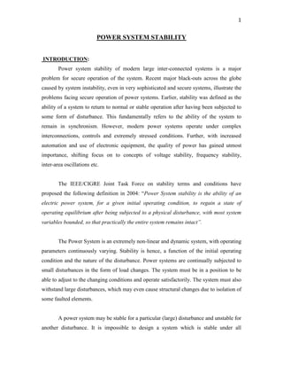
The above assumptions, vastly simplify the equations. A digital computer program for
transient stability analysis can easily include more detailed generator models and effect of
controls, the discussion of which is beyond the scope of present treatment. Studies on the
transient stability of an SMIB system, can shed light on some important aspects of
stability of larger systems. The figure below shows an example of how the clearing
time has an effect on the swing curve of the machine.
15. 15
Modified Euler’s method:
Euler’s method is one of the easiest methods to program for solution of differential
equations using a digital computer . It uses the Taylor’s series expansion, discarding all
second–order and higher–order terms. Modified Euler’s algorithm uses the derivatives at
the beginning of a time step, to predict the values of the dependent variables at the end of
the step (t1 = t0 + Δt). Using the predicted values, the derivatives at the end of the interval
are computed. The average of the two derivatives is used in updating the variables.
Consider two simultaneous differential equations:
),,( tyxf
dt
dx
x
),,( tyxf
dt
dy
y
16. 16
Starting from initial values x0, y0, t0 at the beginning of a time step and a step size h we
solve as follows:
Let
Dx = fx(x0,y0,t0) =
0dt
dx
Dy = fy(x0,y0,t0) =
0dt
dy
valuesPredicted
0
0
hDyy
hDxx
y
P
x
P
DxP =
Pdt
dx
= fx(xP
,yP
,t1)
DyP =
Pdt
dy
= fy(xP
,yP
,t1)
x1 = xo + h
DD xPx
2
y1 = yo + h
DD yPy
2
x 1 and y1 are used in the next iteration. To solve the swing equation by Modified Euler’s
method, it is written as two first order differential equations:
dt
d
M
PP
M
P
dt
d ma sinmax
Starting from an initial value δo, ωo at the beginning of any time step, and choosing a step
size Δt s, the equations to be solved in modified Euler’s are as follows:
0dt
d
= D1 = ωo
0dt
d
= D2 =
M
PPm 0max sin
δP
= δ0 + D1 Δt
ωP
= ω0 + D2 Δt
17. 17
Pdt
d
= D1P = ωP
Pdt
d
= D2P =
M
PP P
m sinmax
δ1 = δ0 +
2
11 PDD
Δt
ω1 = ω0 +
2
22 PDD
Δt
δ1 and ω1 are used as initial values for the successive time step. Numerical errors are
introduced because of discarding higher–order terms in Taylor’s expansion. Errors can be
decreased by choosing smaller values of step size. Too small a step size, will increase
computation, which can lead to large errors due to rounding off. The Runge- Kutta
method which uses higher–order terms is more popular.
Example :A 50 Hz, synchronous generator having inertia constant H = 5.2 MJ/MVA and
dx = 0.3 pu is connected to an infinite bus through a double circuit line as shown in
Fig. 9.21. The reactance of the connecting HT transformer is 0.2 pu and reactance of each
line is 0.4 pu. gE = 1.2 pu and V = 1.0 pu and Pe = 0.8 pu. Obtain the swing curve
using modified Eulers method for a three phase fault occurs at the middle of one of the
transmission lines and is cleared by isolating the faulted line.
18. 18
Solution:
Before fault transfer reactance between generator and infinite bus
XI = 0.3 + 0.2 +
2
4.0
= 0.7 pu
Pmax I =
7.0
0.12.1
= 1.714 pu.
Initial Pe = 0.8 pu = Pm
Initial operating angle δo = sin-1
714.1
8.0
= 27.82o
= 0.485 rad.
When fault occurs at middle of one of the transmission lines, the network and its
reduction is as shown in Fig a to Fig c.
19. 19
The transfer reactance is 1.9 pu.
Pmax II =
9.1
0.12.1
= 0.63 pu
Since there is no outage, Pmax III = Pmax I = 1.714
δmax =
714.1
8.0
sinsin 1
max
1
III
m
P
P
= 2.656 rad
cos δcr =
IIIII
IIIoIIom
PP
PPP
maxmax
maxmaxmaxmax coscos
=
63.0714.1
656.2cos714.1485.0cos63.0485.0656.28.0
=
084.1
5158.15573.07368.1
= – 0.3102
δcr = cos-1
(– 0.3102) = 1.886 rad = 108.07o
with line outage
XIII = 0.3 + 0.2 + 0.4 = 0.9 pu
Pmax III =
9.0
0.12.1
= 1.333 pu
δmax =
333.1
8.0
sin 1
= 2.498 rad
20. 20
Modified Eulers method
δo = 27.82o
= 0.485 rad
ωo = 0.0 rad / sec ( at t = 00
)
Choosing a step size of 0.05 s, the swing is computed. Table a gives the values of the
derivatives and predicted values. Table b gives the initial values δo, ωo and the values at
the end of the interval δ1, ω1. Calculations are illustrated for the time step t = 0.2 s.
δo = 0.761
ωo = 2.072
Pm = 0.8
M =
50
2.5
= 0.0331 s2
/ rad
Pmax (after fault clearance) = 1.333 pu
D1 = 2.072
D2 =
0331.0
)761.0(sin333.18.0
= – 3.604
δP
= 0.761 + ( 2.072 0.05) = 0.865
ωP
= 2.072 + (– 3.604 0.05) = 1.892
D1P = 1.892
D2P =
0331.0
)865.0(sin333.18.0
= – 6.482
δ1 = 0.761 + 05.0
2
892.1072.2
= 0.860
ω1 = 2.072 + 05.0
2
482.6604.3
= 1.82
δ1, ω1 are used as initial values in next time step.
Table a : Calculation of derivatives in modified Euler’s method
22. 22
Runge - Kutta method
In Range - Kutta method, the changes in dependent variables are calculated from
a given set of formulae, derived by using an approximation, to replace a truncated
Taylor’s series expansion. The formulae for the Runge - Kutta fourth order
approximation, for solution of two simultaneous differential equations are given below;
Given
dt
dx
= fx (x, y, t)
dt
dy
= fy (x, y, t)
Starting from initial values x0, y0, t0 and step size h, the updated values are
x1 = x0 +
6
1
(k1 + 2k2 + 2k3 + k4)
y1 = y0 +
6
1
(l1 + 2l2 + 2l3 + l4)
where k1 = fx (x0, y0 ,t0) h
k2 = fx
2
,
2
,
2
0
1
0
1
0
h
t
l
y
k
x h
k3 = fx
2
,
2
,
2
0
2
0
2
0
h
t
l
y
k
x h
k4 = fx (x0 + k3, y0 + l3, t0 + h) h
l1 = fy (x0, y0, t0) h
l2 = fy
2
,
2
,
2
0
1
0
1
0
h
t
l
y
k
x h
l3 = fy
2
,
2
,
2
0
2
0
2
0
h
t
l
y
k
x h
l4 = fy (x0 + k3, y0 + l3, t0 + h) h
The two first order differential equations to be solved to obtain solution for the swing
equation are:
dt
d
= ω
23. 23
M
PP
M
P
dt
d ma sinmax
Starting from initial value δ0, ω0, t0 and a step size of Δt the formulae are as follows
k1 = ω0 Δt
l1 =
M
PPm 0max sin
Δt
k2 =
2
1
0
l
Δt
l2 =
M
k
PPm
2
sin 1
0max
Δt
k3 =
2
2
0
l
Δt
l3 =
M
k
PPm
2
sin 2
0max
Δt
k4 = (ω0 + l3) Δt
l4 =
M
kPPm 30max sin
Δt
δ1 = δ0 +
6
1
[k1 + 2k2 + 2k3 + k4]
ω1 = ω0 +
6
1
[l1 + 2l2 + 2l3 + l4]
Example
Obtain the swing curve for previous example using Runge - Kutta method.
Solution:
δ0 = 27.820
= 0.485 rad.
ω0 = 0.0 rad / sec. ( at t = 0-
)
24. 24
Choosing a step size of 0.05 s, the coefficient k1, k2, k3, k4 and l1, l2, l3, and l4 are
calculated for each time step. The values of δ and ω are then updated. Table a gives the
coefficient for different time steps. Table b gives the starting values δ0, ω0 for a time step
and the updated values δ1, ω1 obtained by Runge - Kutta method. The updated values are
used as initial values for the next time step and process continued. Calculations are
illustrated for the time step t = 0.2 s.
δ0 = 0.756
M = 0.0331 s2
/ rad
ω0 = 2.067
Pm = 0.8
Pmax = 1.333 (after fault is cleared)
k1 = 2.067 × 0.05 = 0.103
l1 = 05.0
0331.0
)756.0(sin333.18.0
= – 0.173
k2 =
2
173.0
067.2 0.05 = 0.099
l2 = 05.0
0331.0
2
103.0
756.0sin333.18.0
= – 0. 246
k3 =
2
246.0
067.2 0.05 = 0.097
l3 = 05.0
0331.0
2
099.0
756.0sin333.18.0
= – 0. 244
k4 = (2.067 – 0.244) 0.05 = 0.091
l4 =
05.0
0331.0
097.0756.0sin333.18.0
= – 0. 308
δ1 = 0.756 +
6
1
[0.103 + 2 × 0.099 + 2 × 0.097 + 0.091] = 0.854
26. 26
0.25 1.333 0.854 1.823 0.936 1.459 53.63
0.30 1.333 0.936 1.459 0.998 1.008 57.18
0.35 1.333 0.998 1.008 1.035 0.502 59.30
0.40 1.333 1.035 0.502 1.046 – 0.029 59.93
0.45 1.333 1.046 – 0.029 1.031 – 0.557 59.07
0.50 1.333 1.031 – 0.557 0.990 – 1.057 56.72
Note: δ0, ω0 indicate values at beginning of interval and δ1, ω1 at end of interval. The
fault is cleared at 0.125 seconds. Pmax = 0.63 at t = 0.1 sec and Pmax = 1.333 at t = 0.15
sec, since fault is already cleared at that time. The swing curves obtained from modified
Euler’s method and Runge - Kutta method are shown in Fig. It can be seen that the two
methods yield very close results.
Fig: : Swing curves with Modified Euler’ and Runge-Kutta methods
27. 27
Milne’s Predictor Corrector method:
The Milne’s formulae for solving two simultaneous differential equations are
given below.
Consider
dt
dx
= fx (x, y, t)
dt
dy
= fy (x, y, t)
With values of x and y known for four consecutive previous times, the predicted value for
n + 1th
time step is given by
nnnn
P
n xxx
h
xx 22
3
4
1231
nnnn
P
n yyy
h
yy 22
3
4
1231
Where x and y are derivatives at the corresponding time step. The corrected values are
xn+1 = 111 4
3
nnnn xxx
h
x
yn+1 = 111 4
3
nnnn yyy
h
y
where 1111 ,, n
P
n
P
nxn tyxfx
1111 ,, n
P
n
P
nyn tyxfy
To start the computations we need four initial values which may be obtained by
modified Euler’s method, Runge - Kutta method or any other numerical method which is
self starting, before applying Milne’s method. The method is applied to the solution of
swing equation as follows:
Define
n
n
dt
d
n
n
n
dt
d
M
PP nm sinmax
nnnn
P
n
t
22
3
4
1231
28. 28
nnnn
P
n
t
22
3
4
1231
δn+1 = δn-1 + 11 4
3
nnn
t
ωn+1 = ωn-1 + 11 4
3
nnn
t
where P
nn 11
M
PP P
nm
n
1max
1
sin
Example
Solve example using Milne’s method.
Solution:
To start the process, we take the first four computations from Range Kutta method
t = 0.0 s δ1 = 0.504 ω1 = 0.759
t = 0.05 s δ2 = 0.559 ω2 = 1.492
t = 0.10 s δ3 = 0.650 ω3 = 2.161
t = 0.15 s δ4 = 0.756 ω4 = 2.067
The corresponding derivatives are calculated using the formulae for n and n . We get
1 = 0.759 1 = 14.97
2 = 1.492 2 = 14.075
3 = 2.161 3 = 12.65
4 =2.067 4 = – 3.46
We now compute δ5 and ω5, at the next time step i.e t = 0.2 s.
43215 22
3
4
tP
= 0.504 + 067.22161.2492.12
3
05.04
= 0.834
P
5 4321 22
3
4
t
29. 29
= 0.759 + )46.3(265.12075.142
3
05.04
= 1.331
5 = 1.331
0331.0
)834.0(sin333.18.0
5
= – 5.657
δ5 = δ3 + 543 4
3
t
= 0.65 + 331.1067.24161.2
3
05.0
= 0.846
ω5 = ω3 + 543 4
3
t
= 2.161 + 657.546.3465.12
3
05.0
= 2.047
5 = ω5 = 2.047
0331.0
)846.0(sin333.18.0
5
= – 5.98
The computations are continued for the next time step in a similar manner.
MULTI MACHINE TRANSIENT STABILITY ANALYSIS
A typical modern power system consists of a few thousands of nodes with heavy
interconnections. Computation simplification and memory reduction have been two
major issues in the development of mathematical models and algorithms for digital
computation of transient stability. In its simplest form, the problem of a multi machine
power system under going a disturbance can be mathematically stated as follows:
0))(( ttxftx I
ceII tttxftx 0))((
tttxftx ceIII ))((
tx is the vector of state variables to describe the differential equations
governing the generator rotor dynamics, dynamics of flux decay and associated generator
30. 30
controller dynamics (like excitation control, PSS, governor control etc). The function fI
describes the dynamics prior to the fault. Since the system is assumed to be in steady
state, all the state variable are constant. If the fault occurs at t = 0, fII describes the
dynamics during fault, till the fault is cleared at time tcl. The post–fault dynamics is
governed by fIII. The state of the system xcl at the end of the fault-on period (at t = tcl)
provides the initial condition for the post–fault network described which determines
whether a system is stable or not after the fault is cleared. Some methods are presented in
the following sections to evaluate multi machine transient stability. However, a detailed
exposition is beyond the scope of the present book.
REDUCED ORDER MODEL
This is the simplest model used in stability analysis and requires minimum data.
The following assumptions are made:
Mechanical power input to each synchronous machine is assumed to be
constant.
Damping is neglected.
Synchronous machines are modeled as constant voltage sources behind
transient reactance.
Loads are represented as constant impedances.
With these assumptions, the multi machine system is represented as in Fig. 9.26.
31. 31
Fig 9.26 Multi machine system
Nodes 1, 2 …… n are introduced in the model and are called internal nodes (the
terminal node is the external node connected to the transmission network). The swing
equations are formed for the various generators using the following steps:
Step 1: All system data is converted to a common base.
Step 2: A prefault load flow is performed, to determine the prefault steady state voltages,
at all the external buses. Using the prefault voltages, the loads are converted into
equivalent shunt admittance, connected between the respective bus and the reference
node. If the complex load at bus i is given by
LiLii QPS
the equivalent admittance is given by
YLi = 22
*
Li
LiLi
Li
iL
V
jQP
V
S
Step 3: The internal voltages are calculated from the terminal voltages, using
32. 32
iidiii IxjVE
=
i
iG
dii
V
S
xjV
*
=
i
iGiG
idi
V
QjP
xjV
'
i is the angle of Ei with respect to Vi. If the angle of Vi is βi, then the angle of
Ei, with respect to common reference is given by iii . PGi and QGi are obtained
from load flow solution.
Step4: The bus admittance matrix Ybus formed to run the load flow is modified to include
the following.
(i) The equivalent shunt load admittance given by, connected between the
respective load bus and the reference node.
(ii) Additional nodes are introduced to represent the generator internal nodes.
Appropriate values of admittances corresponding to dx , connected between
the internal nodes and terminal nodes are used to update the Ybus.
(iii) Ybus corresponding to the faulted network is formed. Generally transient
stability analysis is performed, considering three phase faults, since they are
the most severe. The Ybus during the fault is obtained by setting the elements
of the row and column corresponding to the faulted bus to zero.
(iv) Ybus corresponding to the post–fault network is obtained, taking into account
line outages if any. If the structure of the network does not change, the Ybus
of the post-fault network is same as the prefault network.
Step 5: The admittance form of the network equations is
I = Ybus V
Since loads are all converted into passive admittances, current injections are present only
at the n generator internal nodes. The injections at all other nodes are zero. Therefore, the
current vector I can be partitioned as
I =
0
nI
33. 33
where In is the vector of current injections corresponding to the n generator internal
nodes. Ybus and V are also partitioned appropriately, so that
t
nn
V
E
Y
Y
Y
YI
4
2
3
1
0
where En is the vector of internal emfs of the generators and Vt is the vector of external
bus voltages. From (9.91) we can write
In = Y1 En + Y2 Vt
0 = Y3 En + Y4 Vt
we get
Vt = nEYY 3
1
4
In = 3
1
421 YYYY
En =
Y En
where 3
1
421 YYYYY
is called the reduced admittance matrix and has dimension
nn .
Y gives the relationship between the injected currents and the internal generator
voltages. It is to be noted we have eliminated all nodes except the n internal nodes.
Step 6: The electric power output of the generators are given by
PGi = R [Ei
*
iI .]
Substituting for Ii from (9.94) we get
PGi = )(cosˆ)(sinˆˆ
1
2
jijijijiji
n
ij
iii GBEEGE
(This equation is derived in chapter on load flows)
Step 7: The rotor dynamics representing the swing is now given by
2
2
dt
d
M i
i
= PMi - PGi i = 1………..n
The mechanical power PMi is equal to the pre-fault electrical power output, obtained from
pre-fault load flow solution.
Step 8: The n second order differential equations can be decomposed into 2n first order
differential equations which can be solved by any numerical method .
34. 34
Though reduced order models, also called classical models, require less
computation and memory, their results are not reliable. Further, the interconnections of
the physical network of the system is lost.
FACTORS AFFECTING TRANSIENT STABILITY:
The relative swing of a machine and the critical clearing time are a measure of the
stability of a generating unit. From the swing equation, it is obvious that the generating
units with smaller H, have larger angular swings at any time interval. The maximum
power transfer Pmax =
d
g
x
VE
, where V is the terminal voltage of the generators. Therefore
an increase in dx , would reduce Pmax. Hence, to transfer a given power Pe, the angle δ
would increase since Pe = Pmax sin δ, for a machine with larger dx . This would reduce the
critical clearing time, thus, increasing the probability of losing stability.
Generating units of present day have lower values of H, due to advanced cooling
techniques, which have made it possible to increase the rating of the machines without
significant increase in the size. Modern control schemes like generator excitation control,
Turbine valve control, single-pole operation of circuit breakers and fast-acting circuit
breakers with auto re-closure facility have helped in enhancing overall system stability.
Factors which can improve transient stability are
(i) Reduction of transfer reactance by using parallel lines.
(ii) Reducing transmission line reactance by reducing conductor spacing and
increasing conductor diameter, by using hollow cores.
(iii) Use of bundled conductors.
(iv) Series compensation of the transmission lines with series capacitors. This
also increases the steady state stability limit. However it can lead to problem
of sub-synchronous resonance.
(v) Since most faults are transient, fast acting circuit breakers with rapid
re-closure facility can aid stability.
(vi) The most common type of fault being the single-line-to-ground fault,
selective single pole opening and re-closing can improve stability.
(vii) Use of braking resistors at generator buses. During a fault, there is a sudden
decrease in electric power output of generator. A large resistor, connected at
35. 35
the generator bus, would partially compensate for the load loss and help in
decreasing the acceleration of the generator. The braking resistors are
switched during a fault through circuit breakers and remain for a few cycles
after fault is cleared till system voltage is restored.
(viii) Short circuit current limiters, which can be used to increase transfer
impedance during fault, there by reducing short circuit currents.
(ix) A recent method is fast valving of the turbine where in the mechanical
power is lowered quickly during the fault, and restored once fault is cleared.