ANOVA - Dr. Manu Melwin Joy - School of Management Studies, Cochin University of Science and Technology

Statistical Methods for Engineering Research

Prepared By
Dr. Manu Melwin Joy
Assistant Professor
School of Management Studies
Cochin University of Science and Technology
Kerala, India.
Phone – 9744551114
Mail – manumelwinjoy@cusat.ac.in
Kindly restrict the use of slides for personal purpose.
Please seek permission to reproduce the same in public forms and
presentations.

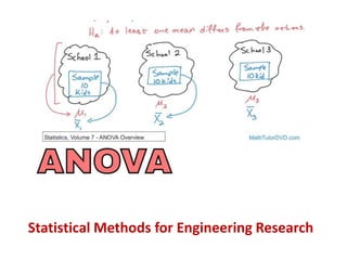
ANOVA
• Analysis of Variance
technique is used to test
whether the mean of
several samples differ
significantly.

• An agronomist may like to know whether yield per acre
will be the same if four different varieties of wheat are
sown in different identical plots.

• A diary farm may like to test whether there is significant
difference between the quality and quantity of milk
obtained from different classes of cattle.

• A business manager may like to find out whether there is
any difference in the average sales by four salesmen.

One Way ANOVA
• In one way ANOVA,
observations are classified
into groups on the basis of
a single criterion.

• For example, suppose we want to study the yield of a crop. This
study is made with respect to the effect of a variable, say fertilizer.
• Here we apply different kinds of fertilizers on different paddy fields
and try to find out difference in the effect of those different kinds of
fertilizers on yield.

One Way ANOVA - Steps
• Step 1
–Find the total of the
values of individual
items in all the
samples.
T = Σ Xij
where i = 1,2,3…….
i = 1,2,3…….

• Step 2
–Correction value is
worked as follows.
Correction value = (T)2
n

• Step 3
–We find the total SS by
squaring all the item
values and taking its
total and subtracting
the correction factors
from it.
Total SS = Σ X2
ij - (T)2
n

• Step 4
– Now we calculate SS
between by obtaining the
square of each sample total
(Tj)2 and dividing each such
value by number of items in
the concerning sample and
totaling it, and from this
total subtracting the
correction factor.
SS between = Σ (Tj)2 - (T)2
n n
Where j = 1,2,3….

• Step 5
–Next SS within is found
out by subtracting the
SS between from total
SS.
SS within = Σ (Xij)2 - Σ (Tj)2
nj

• Step 6
– Calculate MS between by
dividing the sum of squares
for variance between the
sample with degrees of
freedom between samples.
MS between = SS between
(K-1)
Where (k-1) = degree of freedom between samples.

• Step 7
– Calculate MS Within by
for variance within the
sample with degrees of
freedom within samples.
MS Within = SS Within
(n-k)
Where n = total number of items in all the sample i.e. n1+n2+…+nk.
k = total number of samples.
n-k = degrees of freedom within sample.

• Step 8
– Finally, the F-Ration is
calculated as
F – ratio = MS between
MS within

Question 1
• Fifteen students undergoing training are
randomly assigned to three different types of
instruction module. At the end of the training
period, their test scores are as follows.
Module Test 1 Test 2 Test 3 Test 4 Test 5
A 86 79 81 70 84
B 90 76 88 82 89
C 82 68 73 71 81
• Use ANOVA to test that there is no significant
difference in the mean scores of three instruction
modules, using 5 % significance level.

Answer
• H0 : µ1 = µ2 = µ3.
• The null hypothesis assumes no difference in
the mean scores of the three instruction
modules.
• Step (1)
– T = Σ Xij = 1200
• Step (2)
Correction value = (T)2 = (1200*1200)/15 = 96,000
n

• Step (3)
– Total SS = Σ X2
ij - (T)2
n
• (862+ 792+ 812+ 702+ 842+ 902+ 762+ 882+ 822+
892+ 822+ 682+ 732+ 712+ 812) – 96000= 698.
• Step (4)
– SS between = Σ (Tj)2 - (T)2
n n
• (4002)/5 + (4252)/5 + (3752)/5 - 96000 = 250.

• Step (5)
– SS within = Σ (Xij)2 - Σ (Tj)2
nj
– (96698 – 96250) = 448.
• Step (6)
– MS between = SS between = 250/2 = 125
(K-1)
• Step (7)
– MS Within = SS Within = 448/12 = 37.34
(n-k)

• Step (8)
– F – ratio = MS between = 125/ 37.34 = 3.35.
MS within
• Table value of F – ratio is 3.89.
• Since the calculated F-ratio is less than the
table value, the null hypothesis is accepted.
There is no difference in the mean scores of
three instructional modules and whatever is
the difference in their mean scores is
insignificant and due to chance.

Question 2
• In order to test the significance of variation of
retail prices of a commodity in three cities, four
shops were chosen at random from each city and
prices observed in rupees were as follows.
City Shop 1 Shop 2 Shop 3 Shop 4
City A 16 8 12 12
City B 14 10 10 6
City C 4 10 8 10
• Does the data indicate that the prices in three
cities are significantly different?

Answer
• H0 : µ1 = µ2 = µ3.
• The null hypothesis assumes no significant
difference in the prices in three cities.
• Step (1)
– T = Σ Xij = 120
• Step (2)
Correction value = (T)2 = (120*120)/12 = 1200
n

• Step (3)
ij - (T)2
n
• (162+ 82+ 122+ 122+ 142+ 102+ 102+ 62+ 42+ 102+
82+ 102) – 1200= 1320-1200= 120.
• Step (4)
n n
• (482)/4 + (402)/4 + (322)/4 - 1200 = 1232-
1200 = 32.

• Step (5)
nj
– (1320 – 1232) = 88.
• Step (6)
– MS between = SS between = 32/2 = 16.
(K-1)
• Step (7)
– MS Within = SS Within = 88/9 = 9.78.
(n-k)

• Step (8)
MS within
table value, the null hypothesis is accepted. It
is concluded that prices in the three cities are
not significantly different.

Question 3
• A company is interested in knowing if the three
salesmen are performing equally well. The
weekly sales record of the three salesman are :
Salesman Week 1 Week 2 Week 3 Week 4 Week 5
A 300 400 300 500 0
B 600 300 300 400 -
C 700 300 400 600 500
• Does the data indicate that the performance of
the three salesmen are different?

Answer
• H0 : µ1 = µ2 = µ3.
difference in performance of salesmen.
• In order to simplify calculation, we divide each
value by 100 which is a common factor for all.
• Step (1)
– T = Σ Xij = 56
• Step (2)
Correction value = (T)2 = (56*56)/14 = 224
n

• Step (3)
ij - (T)2
n
• (32+ 42+ 32+ 52+ 02+ 62+ 32+ 32+ 42+ 72+ 32+ 42 +
62 + 52) – 224= 264-224= 40.
• Step (4)
n n
• (152)/5 + (162)/4 + (252)/5 - 224 = 10.

• Step (5)
nj
– (264 – 234) = 30.
• Step (6)
(K-1)
• Step (7)
– MS Within = SS Within = 30/11 = 2.73.
(n-k)

• Step (8)
MS within
is concluded that there is no difference
between the performance of three salesmen.

Question 4
• Below are given the yield (in kg) per acre for 5
trial plots of 4 varieties of treatment.
• Carry out an analysis of variance and state your
conclusions.
Plot No I II III IV
1 42 48 68 80
2 50 66 52 94
3 62 68 76 78
4 34 78 64 82
5 52 70 70 66

Answer
• H0 : µ1 = µ2 = µ3 = µ4.
difference in yield because of treatment.
• Step (1)
– T = Σ Xij = 1300
• Step (2)
Correction value = (T)2 = (13002)/20= 84500.
n

• Step (3)
ij - (T)2
n
= (422+ 502+ ……+ 662) - 84500 = 4236
• Step (4)
n n
• (240)2/5 + (330)2/5 + (330)2/5 + (400)2/5 -
84500 = 2580.

• Step (5)
nj
– (88,736 – 87080) = 1656.
• Step (6)
(K-1)
• Step (7)
– MS Within = SS Within = 1656/(20-4) = 103.5.
(n-k)

• Step (8)
MS within
• Table value of F at 5 % level of significance for
(3,16) degrees of freedom is 3.24.
• Since the calculated F-ratio is greater than the
table value, the null hypothesis is rejected. It
is concluded that there is a difference in the
yield created by treatment.

Question 5
• The following table gives the yield of three
varieties.
Varieties I II III IV
1 30 27
2 51 47 48 42
3 44 35 36
• Perform an analysis of variance on this data.

Answer
• H0 : µ1 = µ2 = µ3.
difference in yield of varieties.
• Step (1)
– T = Σ Xij = 480.
• Step (2)
Correction value = (T)2 = (4802)/12= 19200.
n

• Step (3)
ij - (T)2
n
= (302+ 272+ ……+ 362) - 19200 = 578.
• Step (4)
n n
• (99)2/3 + (225)2/5 + (156)2/4 - 19200 = 2580.

• Step (5)
nj
– 578 – 276 = 302.
• Step (6)
(K-1)
• Step (7)
– MS Within = SS Within = 302 / 9 = 33.56.
(n-k)

• Step (8)
– F – ratio = MS between = 138 / 33.56= 4.112.
MS within
is concluded that the yield in the three
varieties are equal.

Answer
• The calculated value of F is less than the table
value of F.
• Therefore the null hypothesis is accepted.
• We accept the hypothesis that the yield in
three varieties are equal.

Question 6
• The following data relate to the yield of four
varieties of wheat each sown, on 5 plots. Find
whether there is a significant difference between
the mean yield of these varieties.
Plot A B C D
1 99 103 109 104
2 101 102 103 100
3 103 100 107 103
4 99 105 97 107
5 98 95 99 106

Answer
• Using coding method, you can use one constant
to minimize calculation. The final value will not
change since it is a ratio. So let us subtract 100
from all the figures.
Plot A B C D
1 -1 3 9 4
2 1 2 3 0
3 3 0 7 3
4 -1 5 -3 7
5 -2 -5 -1 6
0 5 15 20

Answer
• H0 : µ1 = µ2 = µ3.
difference in yield of varieties.
• Step (1)
– T = Σ Xij = 40.
• Step (2)
Correction value = (T)2 = (40)2/20 = 80.
n

• Step (3)
ij - (T)2
n
= (-12+ 12+ ……+ 62) - 80 = 258.
• Step (4)
n n
• (0)2/5 + (5)2/5 + (15)2/5 + (20)2/5 - 80 = 50.

• Step (5)
nj
– 258 – 50 = 208.
• Step (6)
– MS between = SS between = = 50/3 = 16.67.
(K-1)
• Step (7)
– MS Within = SS Within = 208 / 16 = 13.
(n-k)

• Step (8)
– F – ratio = MS between = 16.67 / 13= 1.28.
MS within
is concluded that there is no significant
difference between the mean yield of these
varieties.

Two Way ANOVA
• In two way ANOVA,
observations are classified
into groups on the basis of
a two criterion.

• For example, suppose we want to study the yield of a crop. This study is
made with respect to the effect of two variable, say fertilizer and seed.
• Here we apply different kinds of fertilizers and different kinds of seeds on
different paddy fields and try to find out difference in the effect of those
different kinds of fertilizers and seeds on yield.

Two Way ANOVA - Steps
• Step 1
–Find the total of the
values of individual
items in all the
samples.
T = Σ Xij
where i = 1,2,3…….
i = 1,2,3…….

• Step 2
–Correction value is
worked as follows.
Correction value = (T)2
n

• Step 3
–Work out the sum of
squares of deviation for
total variance by
subtracting the
correction factor from
sum of squared
individual items.
Total SS = Σ X2
ij - (T)2
n
For (c, r-1) degree of freedom

• Step 4
– Sum of squares of
deviation for variance
between the columns is
calculated by subtracting
the correction factor
from sum of square of
column total divided by
number of items in
corresponding column.
SS Column = Σ (Tj)2 - (T)2
nj n
For (c-1) degree of freedom

• Step 5
– Next, sum of squares of
deviation for variance between
rows is calculated by
subtracting the correction
factor from sum of square of
row totals divided by number
of items in the concerning row.
SS Row = Σ (Ti)2 - (T)2
ni n
For (r-1) degree of freedom

• Step 6
– Sum of square of deviation for
residual is found out by subtracting
sum of squares of deviations for
variance between columns and
sum of deviations for variance
between row from sum of squares
of deviation from total variance.
SS Residual = Total SS – (SS between columns + SS between rows)
For (c-1) (r-1) degree of freedom

• Step 7
– Calculate MS Column by
between the column with
degrees of freedom between
columns.
MS column = SS between columns
(c-1)
Where (c-1) = degree of freedom between samples.

• Step 8
– Calculate MS row by dividing
the sum of squares between
the row with degrees of
freedom between row.
MS row = SS between row
(r-1)
Where (r-1) = degree of freedom between samples.

• Step 9
– Calculate MS residual
MS residual = SS residual
(c-1) (r-1)
Where (c-1) (r-1) = degree of freedom between
samples.

• Step 8
– Finally, the F-Ratio is
calculated as
F – ratio = MS between Columns
MS Residual
F – ratio = MS between Rows
MS Residual

Question 7
• Perform a two way ANOVA on the data showing
the number of units of production per day
turned out by 3 different workers using 3
different types of machines.
Workers Machines
A B C
X 5 8 14
Y 5 7 9
Z 8 15 10

Answer
• H01 : There is no significant difference
between the performance of machines.
• H02 : There is no significant difference
between workers.
• Step (1)
– T = Σ Xij = 81.
• Step (2)
n

• Step (3)
ij - (T)2
n
= (52+ 82+ ……+ 102) - 729 = 829-729 = 100.
• Step (4)
– SS between columns = Σ (Tj)2 - (T)2
nj n
• (18)2/3 + (30)2/3 + (33)2/3 - 729 = 42.
• Step (5)
– SS between rows = Σ (Ti)2 - (T)2
ni n
• (27)2/3 + (21)2/3 + (33)2/3 - 729 = 24.

• Step (6)
– Residual SS = Total SS – (SS between column + SS between
rows) = 100 – (42+24) = 34.
• Step (7)
– MS between Column = SS between Columns =
(c-1)
42/2 = 21.
• Step (8)
– MS between row = SS between row =
(r-1)
24/2 = 12.
• Step (9)
– MS residual = SS residual
(c-1)(r-1)
=34/4 = 8.5.

• Step (8)
– F – ratio = MS between Column = 21 / 8.5= 2.47.
MS residual
– F – ratio = MS between row = 12 / 8.5= 1.41.
MS residual
• Table values of F at 5 % level of significance for
• Since the calculated F-ratio is less than the table
value, the null hypothesis is accepted. It is
concluded that there is no significant difference
in performance of machine and that of workers.

Question 8
• Perform a two way ANOVA on the data given
below which shows four levels of prices and
three advertisement campaigns as treatments
and the figures show the sales in lakh rupees.
Ad Campaign Price levels
I II III IV
A 38 40 41 39
B 45 42 49 36
C 40 38 42 42

• The calculation can be made easier by using the
coding method and subtracting 40 from each
value so that the data set now comes out as
follows:
Ad Campaign Price levels
I II III IV
A -2 0 1 -1
B 5 2 9 -4
C 0 -2 2 2

Answer
• H01 : There is no significant difference in price
level.
• H02 : There is no significant difference in
advertisement campaign.
• Step (1)
– T = Σ Xij = 12.
• Step (2)
n

• Step (3)
ij - (T)2
n
= (-22+ 52+ ……+ 22) - 12 = 144-12 = 132.
• Step (4)
nj n
• (3)2/3 + (0)2/3 + (12)2/3 + (-3)2/3 - 12 = 42.
• Step (5)
ni n
• (-2)2/4 + (12)2/4 + (2)2/4 - 12 = 26.

• Step (6)
– Residual SS = Total SS – (SS between column + SS between
rows) = 132 – (42+26) = 64.
• Step (7)
(c-1)
42/3 = 14.
• Step (8)
(r-1)
26/2 = 13.
• Step (9)
– MS residual= SS residual
(c-1)(r-1)
64/6 = 10.67.

• Step (8)
MS residual
– F – ratio = MS between row = 13 / 10.67= 1.218.
MS residual
• Table values of F at 5 % level of significance for (3,6)
and (2,6) degrees of freedom are 4.76 and 5.14.
• Since the calculated F-ratio is less than the table value,
the null hypothesis is accepted. It is concluded that
there is no significant difference in between price
levels as well as between advertising campaigns.

ANOVA with repeated values
• The two way ANOVA with repeated values
involves the same steps as one without
repeated values except that in this case, the
interaction variation is worked out.

Question 9
• Is the interaction variation significant in case of
the following information concerning mileage
based on different brands of gasoline and cars.
Cars Brands of gasoline
X Y Z
A 12 10 9
12 9 11
B 12 7 10
11 8 11
C 10 11 8
11 11 7

Answer
• H01 : There is a significant interaction between
cars and brands of gasoline.
• Step (1)
– T = Σ Xij = 180.
• Step (2)
n

• Step (3)
ij - (T)2
n
= (122+ 122+ ……+ 72) - 1800 = 46.
• Step (4)
nj n
• (68)2/6 + (56)2/6 + (56)2/6 - 1800 = 16.01.
• Step (5)
ni n
• (63)2/6 + (59)2/6 + (58)2/3 - 1800 = 2.34.

• Step (6)
– SS within is next calculated by subtracting each
item within a group with its mean .
– SS within = (12-12)2 + (12-12)2 + (12-11.5)2 + (11-
11.5)2 + (10-10.5)2 + (11-10.5)2 + …..
+ (8-7.5) 2 + (7.5 – 7) 2= 5.
• Step (7)
– SS interaction variation is the left over variation
calculated by deducing the sum of SS column, SS
rows and SS within from SS total.
– SS interaction = SS total – (Ss column+ SS row + SS
within) = 46 – (16.01 + 2.34 + 5) = 22.65.

• The degree of freedom for various sources of
variance are as follows.
– D.F for total SS = n-1 = 18-1 = 17.
– D.F for SS between column = c-1 = 3-1 = 2.
– D.F for SS between rows = r-1 - 3-1 =2.
– D.F for SS within = n-k = 18-9 = 9.
– D.F for interaction = (n-1) – ((c-1) + (r-1) + (n-k)) =
17- (2+2+9) = 4

• Step (7)
(c-1)
16.01/2 = 8.
• Step (8)
(r-1)
2.34/2 = 1.17.
• Step (9)
– MS Within = SS Within
(n-k)
=5/9 = 0.56.
• Step (10)
– MS Interaction = SS Interaction
(n-1) – ((c-1) + (r-1) + (n-k))
=22.65/4 = 5.66.

• Step (8)
MS Within
– F – ratio = MS between row = 1.17 / 0.56= 2.09.
MS Within
– F – ratio = MS Interaction = 5.66 / 0.56= 10.1.
MS Within
• Table values of F at 5 % level of significance for (2,9) , (2,9) and (4,9)
degrees of freedom are 4.26, 4.26 and 3.63.
• Since the calculated F-ratio for interaction matrix is higher than the
table value, the null hypothesis is rejected. In other words, there is
significant interaction between cars and brand of gasoline, hence
column and row effect results are of no use for researcher.

ANOVA - Dr. Manu Melwin Joy - School of Management Studies, Cochin University of Science and Technology

ANOVA - Dr. Manu Melwin Joy - School of Management Studies, Cochin University of Science and Technology

Recommended

Recommended

More Related Content

What's hot

What's hot (20)

Similar to ANOVA - Dr. Manu Melwin Joy - School of Management Studies, Cochin University of Science and Technology

Similar to ANOVA - Dr. Manu Melwin Joy - School of Management Studies, Cochin University of Science and Technology (20)

More from manumelwin

More from manumelwin (20)

Recently uploaded

Recently uploaded (20)

ANOVA - Dr. Manu Melwin Joy - School of Management Studies, Cochin University of Science and Technology