1. Surface hydrology of an arctic ecosystem: multi-scale analysis of
a flooding and draining experiment using spectral reflectance
INTRODUCTION METHODS RESULTS RESULTS
In the Arctic, soil moisture and surface hydrology control plant Presence of surface water in the study area
community composition and ecosystem processes such as land- Table 1. Results of regressions between EWT, WBI, NDSWI-log,
affected reflectance spectra markedly. The NDSWI-linear and water table depth for July 18, 23, 28, August 4 and
atmosphere carbon and water exchange and energy balance. biggest change was observed in the near-
Investigating how climate change in this region will affect surface August 9, 2008. Y = water table depth, x = index value. Here R2 values
infrared , and the least change was observed are calculated from all dates combined.
hydrology and subsequent biotic, atmospheric and climatic feedbacks, in the blue spectral region Title 2).
Section (Fig.
particularly the potential for the large arctic soil organic carbon pool to
be mobilized to the atmosphere as greenhouse gases, could be key to Section text here. Section text here. Section text here.
understanding the future state of the Arctic and Earth systems. Section text here. Section text here. Section text here.
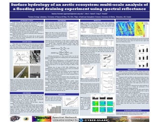
Figure 2. The effect of surface water (expressed here.
Section text here. Section text as
Improved methods are needed for monitoring surface hydrology at surface water cover) on reflectance spectra. Each
large spatial scales in the Arctic. field spectrum is compared to a modeled reflectance Table 2. Results of the regressions between EWT, WBI, NDSWI-log,
Despite this, there have been few studies that use optical remote spectra using spectral mixture analysis for the same NDSWI-linear and Percent Surface Water Cover (surface water cover)
sensing to explore how surface hydrological state can be quantified percent of standing surface water.
for July18, 2008. Y = Percent surface water cover, x = index value. Here Figure 9. Spatial patterns of elevation (figures 8a to 8c), measured WTD through
using remote sensing technologies.
R2 values are calculated from all dates combined. the season (figures 8d to 8f) and modeled WTD through the season (figures 8g to
Following the non-responsiveness of blue region to standing surface 8i) for all three tramlines (north, central and south, from left to right in this
STUDY SITE water and responses of the IR region to the surface standing water (Fig order) for the 2008 growing season.
3), a spectral index, normalized difference surface water index
Water tables were manipulated in a thaw-lake basin to investigate
(NDSWI), was derived using two narrow wavebands at 460nm and Figure 10. Comparison of average NDSWI-
the impact of variation of soil moisture on land-atmosphere carbon, linear mapped to different sampling footprint
1000nm as follows:
water and energy balance as part of NSF supported Biocomplexity NDSWI-log showed the strongest relationship among all four indices areas using Quickbird 2002 and 2008 images.
project at Barrow Environmental Observatory in Barrow, Alaska (Fig1). R460 − R1000 Error bars represent one standard deviation. ‘*’
NDSWI− linear= → (1) tested and was also able to predict the measured water table depth for the
R460 + R1000 snow free time of the growing season. Therefore, from now on we will
- Indicates significant difference (P < 0.05, T-
Test) between years (2002 and 2008) for a
use this index to test its ability over space and time to predict the water
ln(R1000) − ln(R460) table depth along the study area.
given sampling area (tramline footprint, flux
NDSWI− log = → (2) tower footprint, treatment basin) and treatment
ln(R1000) + ln(R460) Figure 5. Models that predict water table depth 5a
(flooded, drained, control). A/B/C - Indicates
(all points), surface water depth (solid circles), significant difference/similarity (P < 0.05,
Following determination of which spectral index was the best
below-ground water (open circles) (panel 5a), Univariate ANOVA) between treatments
predictor of WTD throughout the sampling period, the model predicting and surface water cover (solid circles, panel 5b) (flooded, drained, control) in a given year and
WTD was refined. from NDSWI-log. This model was derived type of sampling area. I/II/III – Indicates
Two other indices, WBI (Pinuelas et. al 1997) and EWT (Sims and using data from July 18, 23, 28, August 4 and 5b significant difference/similarity (P < 0.05,
Gamon, 2003) alongwith NDSWI-linear and NDSWI-log were tested August 9, 2008. Modeled surface water cover Kolomogorov-Smirnof test) between sampling
using spectral mixture analysis are also shown areas (tramline footprint, flux tower footprint,
for their ability to predict the water table depths along the tramline
(open circles, panel 5b). treatment basin) within a given treatment and
using data from July 18, 23, 28, August 4 and August 9, 2008 (n = 450) year.
(Table 1).
Similarly, July 18 values of EWT, WBI, NDSWI-linear, and
NDSWI-log were correlated with percent surface water cover estimated
from digital image analysis (n = 90) (Table 2). DISCUSSION
Seasonal WTD trends for each tramline were then modeled and NDSWI was able to accurately estimate standing surface water
compared to measured WTD, both seasonally and as a direct 1:1 depth in an experimental flooding and draining experiment situated in
comparison to determine if the model over or under-estimated WTD in a vegetated thaw lake basin on the Arctic Coastal Plain of northern
each of the experimental treatments. Alaska.
Mosaic plots combining all treatment dates and positions were Compared to EWT and WBI, two other spectral indices that have
derived to assess the spatio-temporal behavior of the model along each Figure 6. Modeled vs. measured water table been widely used to estimate surface hydrological properties using
Figure 1. Location of Barrow Environmental Observatory (BEO) near Barrow, tramline and throughout the sampling period. depth for all the three tramlines for 2008 snow remote sensing (Penuelas et a. 1993, Gao and Goetz 1995, Roberts et
Alaska (Fig. 1a). Figure 1b shows the location of the study area. The experimental Two high-spatial resolution multispectral satellite images free period using a model derived for July 18th. al. 1997, Sims and Gamon 2003, Green et al. 2006), NDSWI was a
design of the Biocomplexity Experiment includes experimentally flooded (north) (QuickBird, Digital Globe, Longmont, Colorado, USA) acquired on better predictor of standing surface water depth, percent water cover,
and drained (central) treatments, and a control section (south) shown by the letters August 2, 2002 and July 27, 2008, were used to scale NDSWI to the Figure 7. Seasonal patterns of mean measured
F, D and C respectively (Fig 1b). Watersheds for each treatment and the inundated and WTD within the study area..
landscape level for pre- (2002) and post- (2008) treatment years (Fig 8). water table depth along the three tramlines and The capacity of NDSWI to characterize the surface hydrology of
basin areas are highlighted (Fig 1b). The straight lines (Fig 1b) indicate the three mean modeled water table depth for each
sampling transects (“tramlines”) (Fig 1c) and the three pie-shaped semi circles
The sampling footprints of the tramlines and flux towers and the the study area enabled us to evaluate the performance of the
inundated basin of the experimental area were delineated in GIS for tramline. Panels 8a, 8b and 8c show flooded
indicate idealized footprints of the three flux tower footprints associated with the (north), drained (central) and control (south) experimental flooding and draining experiment.
experiment. Figure 1d shows the robotic cart used for collecting hyperspectral each treatment area and statistics were applied to find significant A distinct advantage of NDSWI over the other spectral indices
treatments respectively. The peak in between
reflectance data. differences between the treatments (Fig 10). day 210 and day 215 in the drained and control tested in this study is that it can be readily calculated from a range of
treatments indicates a snow fall event for that publicly available satellite remote sensing platforms.
METHODS particular day. In conclusion, our study has addressed a critical need in the
RESULTS Arctic terrestrial sciences – an improved capacity to detect and
Hyperspectral reflectance data in the visible-nearIR region of the
spectrum were collected using a portable spectrometer onboard a Figure 3. R2 values for wavelength vs. monitor surface hydrological properties associated with important
Figure 8. Spatial patterns ecological processes and phenomena. Our goal to develop a spectral
robotic tram system (Fig. 1c and 1d) consisting of three 300 meter long water table depth, surface water depth
of microptopography
tramlines in east – west direction in the three experimental and surface water cover. Data for this index from optical remote sensing tools that could be used to estimate
(Fig. 8a to 8c), seasonal
manipulation sections (Fig. 1b) for June – August, 2008. analysis was collected on July 18 2008.
measured WTD (Fig. 8d
standing surface water depth, and changes in surface hydrology at
Water table depths were collected every ten meters along the to 8f) and modeled multiple spatial and temporal scales. NDSWI out-performed other
tramlines for every reflectance measurements. seasonal WTD (Fig. 8g spectral indices that have been used to estimate similar surface
Photos of each tramline footprint (matching the optical sampling to 8i) for all three properties.
tramlines for the 2008
areas) were acquired on July 18, 2008, using a digital camera (Coolpix
snow-free season
5400, Nikon) that was mounted on the boom of the robotic cart and (flooded, drained,
triggered manually using an electronic shutter cable. The photo Figure 4. R2 values for the prediction of control, left to right).
locations were also adjacent to water table depth measurements, water table depth from NDSWI for all ACKNOWLEDGEMENT
allowing direct comparison with water table depth and surface water tramlines comparing linear and log
depth measurements. versions of the index for different dates National Science Foundation, Barrow Arctic Science Consortium, UIC,
in 2008. CH2M Hill Polar Resources, Systems Ecology Lab at UTEP.