1. Timing Advances
Access Burst Duration of a Bit Propagation Delay Max Cell Size Determining a TA Distance of a TA
Home
`
Introduction
A Timing Advance (TA) is used to compensate for the propagation delay as the signal travels between the Mobile Station (MS) and Base
Transceiver Station (BTS). The Base Station System (BSS) assigns the TA to the MS based on how far away it perceives the MS to be.
Determination of the TA is a normally a function of the Base Station Controller (BSC), bit this function can be handled anywhere in the BSS,
depending on the manufacturer.
Time Division Multiple Access (TDMA) requires precise timing of both the MS and BTS systems. When a MS wants to gain access to the
network, it sends an access burst on the RACH. The further away the MS is from the BTS, the longer it will take the access burst to arrive at the
BTS, due to propagation delay. Eventually there comes a certain point where the access burst would arrive so late that it would occur outside its
designated timeslot and would interfere with the next time slot.
Access Burst
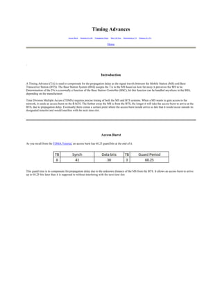
As you recall from the TDMA Tutorial, an access burst has 68.25 guard bits at the end of it.
This guard time is to compensate for propagation delay due to the unknown distance of the MS from the BTS. It allows an access burst to arrive
up to 68.25 bits later than it is supposed to without interfering with the next time slot.

2. 68.25 bits doesnt mean much to us in the sense of time, so we must convert 68.25 bits into a frame of time. To do this, it is necessary to calculate
the duration of a single bit, the duration is the amount of time it would take to transmit a single bit.
[Back to Top]
Duration of a Single Bit
As you recall, GSM uses Gaussian Minimum Shift Keying (GMSK) as its modulation method, which has a data throughput of 270.833
kilobits/second (kb/s).
Calculate duration of a bit.
Description Formula Result
Convert kilobits to bits 270.833 kb × 1000 270,833 bits
Calculate seconds per bit 1 sec ÷ 270,833 bits .00000369 seconds
Convert seconds to microseconds .00000369 sec × 1,000,000 3.69 µs
So now we know that it takes 3.69µs to transmit a single bit.
[Back to Top]
Propagation Delay
Now, if an access burst has a guard period of 68.25 bits this results in a maximum delay time of approximately 252µs (3.69µs × 68.25 bits). This
means that a signal from the MS could arrive up to 252µs after it is expected and it would not interfere with the next time slot.

3. The next step is to calculate how far away a mobile station would have to be for a radio wave to take 252µs to arrive at the BTS, this would be
the theoretical maximum distance that a MS could transmit and still arrive within the correct time slot.
Using the speed of light, we can calculate the distance that a radio wave would travel in a given time frame. The speed of light (c) is 300,000
km/s.
Description Formula Result
Convert km to m 300,000km × 1000 300,000,000m
Convert m/s to m/µs 300,000,000 ÷ 1,000,000 300 m/µs
Calculate distance for 252µs 300 m/µs × 252µs 75600m
Convert m to km 75,600m ÷ 1000 75.6km
So, we can determine that a MS could theoretically be up to 75.6km away from a BTS when it transmits its access burst and still not interfere
with the next time slot.
However, we must take into account that the MS synchronizes with the signal it receives from the BTS. We must account for the time it takes for
the synchronization signal to travel from the BTS to the MS. When the MS receives the synchronization signal from the BTS, it has no way of
determining how far away it is from the BTS. So, when the MS receives the syncronization signal on the SCH, it synchronizes its time with the
timing of the system. However, by the time the signal arrives at the MS, the timing of the BTS has already progressed some. Therefore, the
timing of the MS will now be behind the timing of the BTS for an amount of time equal to the travel time from the BTS to the MS.
For example, if a MS were exactly 75.6km away from the BTS, then it would take 252µs for the signal to travel from the BTS to the MS.

4. The MS would then synchronize with this timing and send its access burst on the RACH. It would take 252µs for this signal to return to the BTS.
The total round trip time would be 504µs. So, by the time the signal from the MS arrives at the BTS, it will be 504µs behind the timing of the
BTS. 504µs equals about 136.5 bits.
The 68.25 bits of guard time would absorb some of the delay of 136.5 bits, but the access burst would still cut into the next time slot a whopping
68.25bits.

5. [Back to Top]
Maximum Size of a Cell
In order to compensate for the two-way trip of the radio link, we must divide the maximum delay distance in half. So, dividing 75.6km in half, we
get approximately 37.8 km. If a MS is further out than 37.8km and transmits an access burst it will most likely interfere with the following time
slot. Any distance less than 37.8km and the access burst should arrive within the guard time allowed for an access burst and it will not interfere
with the next time slot.
In GSM, the maximum distance of a cell is standardized at 35km. This is due mainly to the number of timing advances allowed in GSM, which is
explained below.
[Back to Top]
How a BSS Determines a Timing Advance
In order to determine the propagation delay between the MS and the BSS, the BSS uses the synchronization sequence within an access burst. The
BSS examines the synchronization sequence and sees how long it arrived after the time that it expected it to arrive. As we learned from above, the
duration of a single bit is approximately 3.69µs. So, if the BSS sees that the synchronization is late by a single bit, then it knows that the
propagation delay is 3.69µs. This is how the BSS knows which TA to send to the MS.

6. For each 3.69µs of propagation delay, the TA will be incremented by 1. If the delay is less than 3.69µs, no adjustment is used and this is known
as TA0. For every TA, the MS will start its transmission 3.69µs (or one bit) early. Each TA really corresponds to a range of propagation delay.
Each TA is essentially equal to a 1-bit delay detected in the synchronization sequence.
TA From To
0 0µs 3.69µs
1 3.69µs 7.38µs
2 7.38µs 11.07µs
3 11.07µs 14.76µs
... ... ...
63 232.47µs 236.16µs
[Back to Top]
The Distance of a Timing Advance
When calculating the distances involved for each TA, we must remember that the total propagation delay accounts for a two-way trip of the radio
wave. The first leg is the synchronization signal traveling from the BTS to the MS, and the second leg is the access burst traveling from the MS to
the BTS. If we want to know the true distance of the MS from the BTS, we must divide the total propagation delay in half.
For example, if the BSS determines the total propagation delay to be 3.69µs, we can determine the distance of the MS from the BTS.
Description Formula Result
Determine one-way propagation time 3.69µs ÷ 2 1.845µs
Calculate distance
300 m/µs × 1.845µs 553.5m
(using speed of light.)

7. We determined earlier that for each propagation delay of 3.69µs the TA is inceremented by one. We just learned that a propagation delay of
3.69µs equals a one-way distance of 553.5 meters. So, we see that each TA is equal to a distance of 553.5 meters from the tower. Starting from
the BTS (0 meters) a new TA will start every 553.5m.
TA Ring Start End
0 0 553.5m
1 553.5m 1107m
2 1107m 1660.5m
3 1660.5m 2214m
... ... ...
63 34.87km 35.42km
The TA becomes very important when the MS switches over to using a normal burst in order to transmit data. The normal burst does not have the
68.25 bits of guard time. The normal burst only has 8.25 bits of guard time, so the MS must transmit with more precise timing. With a guard time
of 8.25 bits, the normal burst can only be received up to 30.44µs late and not interfere with the next time slot. Because of the two-way trip of the

8. radio signal, if the MS transmits more than 15.22µs after it is supposed to then it will interfere with the next time slot.
Access Burst Duration of a Bit Propagation Delay Max Cell Size Determining a TA Distance of a TA
Introduction Architecture TDMA Logical Channels Authentication & Encryption Timing Advances Speech Encoding GSM Events Cell Selection/Reselection
Updates Sitemap Contact Me
Home

9. Cell Selection and Reselection
Signal Strength RXQUAL Cell Selection and Reselection C1 C2 Cell Reselection Offset Cell Reselection
Hysteresis Cell Bar Access Cell Bar Qualifier
Home
Note: This tutorial is intended for people that have a good basic understanding of GSM fundamentals. It
may be necessary to review Introduction to GSM and Network Architecture before reading this tutorial.
There are many factors involved in maintaining the radio link (Um interface) between the Mobile Station
(MS) and the Base Transceiver Station (BTS). As the MS moves throughout the network the signal
strength of the BTS will increase and decrease and the MS will have to continuously monitor the signal
strengths of nearby towers and update which BTS's it camps on. This page covers all of the parameters
that the MS and network will use in order to ensure the the MS chooses the strongest tower to monitor
and other network considerations.
Signal Strength
The first and arguably most important consideration in radio link management is signal strength. In GSM
(and most other RF communications) the standard measure of signal strength is dBm (decibels in
milliwatts). The term received signal strength indicator (RSSI) is often used but in GSM the
term received-signal level(RXLEV) is preferred. The distinction is that the term RSSI was generally used
on analog networks and RXLEV is used on digital networks. On this website RSSI will be used for
general reference to signal strength and RXLEV for the actual value that is passed over the network.
RXLEV
RXLEV is a number from 0 to 63 that corresponds to a dBm value range. 0 represents the weakest signal
and 63 the strongest.

10. RSSI below -110 dBm are generally considered unreadable in GSM. RSSI in the area of -50 dBm are
rarely seen and would indicate that the MS is right next to the BTS. The main factor that affects RSSI is
distance from the tower. However, other factors such as terrain, elevation, and large objects such as
buildings can dampen signal strength.
RXQUAL
Although a strong RSSI is desirable, it does not guarantee a quality signal. RXQUAL is a value that
represents the quality of the received signal. The MS determines the Bit Error Rate (BER) of the signal
and reports it back to the network. The BER is simply a percentage of the number of bits it receives that
did not pass error checking. The bits may have been garbled along the RF path or lost due to fading or
interference. The higher the BER the lower the signal quality. RXQUAL is given as a number from 0 to 7
and represents a percentage range of BER.

11. Cell Selection and Reselection
Cell selection refers to the initial registration that a MS will make with a network. This normally only
occurs when the phone powers up or when the MS roams from one network to another.
Cell reselection refers to the process of a MS choosing a new cell to monitor once it has already registered
and is camped on a cell. It is important to distinguish that selection and reselection are done by the MS
itself and not governed by the network. The network would only be responsible for this function when the
MS is in aTraffic Channel (TCH). When the MS reselects a new cell it will not inform the network that it
has done so unless that new cell is in a new Location Area (LA).
There are many parameters involved in selection and reselection of a new cell. The MS must ensure it is
getting the best signal and the network must ensure that the MS does not cause unneeded strain on the
network by switching cells when unnecessary or undesired.
C1
C1 is the path-loss parameter that is used to determine the strongest cell for selection. The MS will
calculate a C1 for each tower it can see and select the cell tower with the highest C1. The C1 uses the
following parameters for calculation:
The formula for calculating C1 is given as:
C1 = (A) - Max(B,0)
where:
A = (RXLEV - RLAM)
B = MS Transmit Power Max CCH -Max RF Output of MS
At first this may seem complicated but if we examine the various parameters and how they affect the C1
score then it becomes more clear.
A - This value is merely a dB value for the difference between what RSSI is required to select that cell
and what signal strength the MS sees the tower at. If the RLAM is -110dB and the MS sees the tower at -

12. 90dB then the value of A is 20dB. The higher the value of A the higher the C1 and the more attractive this
tower will be to the MS.
B - Just because a MS can receive a tower's signal does not mean that the MS has enough power to reach
that tower. The tower tells the MS what maximum power level that the MS may use to transmit to that
tower. If the phone is capable of transmitting at this power than there is no problem. However, what if the
phone can not transmit at that power level? The signal from the MS may not have enough power to reach
the tower. Any lack in transmitting power of the MS must be taken into account when calculating C1. B is
essentially the value of this difference. Let's say a cell tower requires the MS to be able to transmit at a
30dB power level but this MS is only capable of transmitting at 26dB. In this case the value of B would
be 4dB. This value is subtracted from the value of A which has the result of lowering the value of C1. If
the MS is capable of transmitting at the required power or higher then B will be zero and no adjustments
to C1 will be made.
In summary, the two main factors in determining C1 are the strength of the received signal and the
transmission power the MS is capable of. C1 alone is only used for cell selection. When a MS is already
camped on a cell and it wants to move to another cell it will reselect it. Cell reselection uses a different
criteria C2.
C2
C2 is the parameter used for cell reselection. Once a MS is camped on a cell it will continuously monitor
the strength of neighbor cells. Every BCCH sends out aBCCH Allocation (BA) List. This is a list of
neighbor cells (ARFCNs) that the MS must monitor while camped on a particular cell. The MS will
monitor these ARFCNs for signal strength and only reselect a cell that is on this list. The MS will
calculate a C2 value for each cell on the BA list. The cell tower with the highest C2 wins and the MS will
move to that cell and camp on it. Keep in mind the C2 is calculated by the MS and the MS decides which
cell tower to camp on. The cell that the MS camps on is known as the serving cell. As long as the losing
cell and the gaining cell are both in the same Location Area the MS will not notify the network that is is
selecting a new cell. The MS only needs to notify the network if it is reselecting the cell that is in a new
location area in which case it will do alocation update.

13. The C2 is calculated using the following parameters:
The formula for calculating C2 is:
C2 = C1 + CRO - (Temp_Offset * H)
H = 1 if the MS has been monitoring a particular cell for less than the penalty time.
H = 0 if the MS has been monitoring the particular cell for longer than the penalty time.
H = 0 if the particular cell is the serving cell (the one the MS is currently camped on).
Let's look at an example to see how the temporary offset works. The following chart shows two example
cell towers and values for C1 and C2 parameters. The time progresses as the MS moves away from cell A
and towards cell B. For sake of simplicity, we are assuming that the MS can transmit at the max power
allowed and that neither cell is using CRO.
0 seconds - The MS is camped on cell A. The MS calculates the C2 value as 38. Since the RXLEV for
cell B is not above the RLAM the C1 (and C2) are below 0. A MS will not select a cell with a C1 below 0
and it will not reselect a cell with a C2 below 0.
10 seconds - The RXLEV for cell B meets the minimum threshold (RLAM). The MS starts a timer as
soon as it puts it on its strongest neighbor list. The penalty time for cell B is 40 seconds, so for the first 40

14. seconds that cell B is on the strongest neighbor list it will apply the temporary offset to the C2 value.
After including the offset, the C2 for cell B is -20 dBm.
20 seconds - The C2 for cell A continues to drop as the C2 for cell B continues to rise. With a C2 of 25,
cell A is still the most attractive.
30 seconds - Cell A drops to a C2 of 21 and cell B has a C2 of -5.
40 seconds - Cell A drops to a C2 of 18. Cell B rises to a C2 of 3. Notice here that if it were not for the
temporary offset, the C2 for cell B would be at 23. At this point the MS would normally reselect cell B.
However, due to the temporary offset, cell A is still the most attractive.
50 seconds - At this point the penalty time for cell B has expired and the temporary offset is no longer
applied. The C2 for cell B raises from 3 to 27. The C2 for cell B wins over the C2 for cell A and the MS
reselects cell B.
The temporary offset would be used if the network wanted to discourage mobile stations from reselecting
a cell as soon as the MS saw it. This is commonly found in pico-cells. This forces a MS to be in the area
of the cell for a certain period before reselecting it. It prevents mobile stations that just happen to be
passing by from reselecting the cell. In order to reselect the cell, the MS must be in the area for a certain
period of time or be close enough that the RXLEV overcomes the negative offset value.
Cell Reselection Offset (CRO) - CRO is a value from 0 to 63. Each step represents a 2 dBm step (0 to
126 dBm). This value is added to C1. A higher CRO value will make the cell tower more attractive to the
MS. The higher the CRO, the more attractive the cell will be. The network might assign a CRO value to a
cell if the network wanted to encourage mobile stations to utilize that cell. The network might want to do
this in order to reduce the load on other cells during times of high traffic volume or to force MS's to a
certain band.
Neighbor List - The neighbor list is a list of the 6 strongest cells that the MS can see. The RXLEV for
these cells is transmitted in a measurement report from the MS to the BTS on the SACCH whenever the
MS has been allocated an SDCCH or a TCH. The BSC and MSC use these measurements to determine if
the MS needs to move to a different cell. Whenever a cell is in an active SDCCH or TCH the network will
always manage the handoff. The MS will only move from one cell to another by itself when it is in idle
mode.

15. Cell Reselection Hysteresis (CRH)
When a MS reselects a new cell it does not need to notify the network unless that new cell is in a
different Location Area. When a MS moves into a new location area it must do a location update which
generates signal messaging between the BTS, BSC, MSC, VLR, and HLR. If a MS is located along the
border of two location areas then it will see cells in both location areas. A MS along the borderline might
reselect a cell in one location area and then a few minutes later reselect a cell in the other location area
and continuously bounce back and forth between location areas generating too much signaling overhead
and putting strain on the network.
In order to mitigate this problem the CRH is used. It is a value that is similar to the temporary offset value
of C2. CRH is applied to C2 when the desired cell is in a different location area. This results in making
the cell in this different location area less desirable to the MS. The MS must move close enough to the
new location area to overcome the offset thus ensuring the MS is truly close enough to the new location
area to warrant a location update. Once the MS reselects the cell in the new location area it will perform a
location update. The MS will then apply the CRH value to all cells it sees in the old location area which
will make them less attractive to the MS and ensure the MS does not continually bounce back and forth
between two location areas.
Cell Bar Access (CBA)
Cell Bar Access is a single bit (0 or 1) value sent down on the BCCH. If CBA is set to 1 then MS's are not
allowed to select that cell. If the value is set to 0 then MS's may select it. CBA would be used on umbrella
cells in order to prevent MS's from selecting it. The umbrella cell would be reserved for when the network
needs to manage high levels of traffic. This gives the network total control of access to the umbrella cell.
Cell Bar Qualifier (CBQ)
This value is similar to the CBA but it applies to reselection. A cell that has CBQ set to 1 does not allow
MS's to reselect it. CBQ set to 0 allows normal access to that cell.
Signal Strength RXQUAL Cell Selection and Reselection C1 C2 Cell Reselection Offset Cell Reselection
Hysteresis Cell Bar Access Cell Bar Qualifier
Introduction Architecture TDMA Logical Channels Authentication & Encryption Timing Advances Speech
Encoding GSM Events Cell Selection/Reselection
Updates Sitemap Contact Me
Home