Ch.08

CONTENTS
CONTENTS

174 l Theory of Machines

Features
eatur
tures
Warping Machine

1. Introduction.
Acceleration
8
2. Acceleration Diagram for a
Link.
3. Acceleration of a Point on a
in Mechanisms
Link.
4. Acceleration in the Slider 8.1. Introduction
Introduction
Crank Mechanism.
We have discussed in the previous chapter the
5. Coriolis Component of
Acceleration.
velocities of various points in the mechanisms. Now we shall
discuss the acceleration of points in the mechanisms. The
acceleration analysis plays a very important role in the
development of machines and mechanisms.

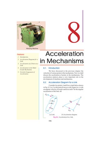
8.2. Acceleration Diagram for a Link
Consider two points A and B on a rigid link as shown
in Fig. 8.1 (a). Let the point B moves with respect to A, with
an angular velocity of ω rad/s and let α rad/s2 be the angular
acceleration of the link AB.

(a) Link. (b) Acceleration diagram.
Fig. 8.1. Acceleration for a link.

174

CONTENTS
CONTENTS

Chapter 8 : Acceleration in Mechanisms l 175
We have already discussed that acceleration of a particle whose velocity changes both in
magnitude and direction at any instant has the following two components :
1. The centripetal or radial component, which is perpendicular to the velocity of the
particle at the given instant.
2. The tangential component, which is parallel to the velocity of the particle at the given
instant.
Thus for a link A B, the velocity of point B with respect to A (i.e. vBA) is perpendicular to the
link A B as shown in Fig. 8.1 (a). Since the point B moves with respect to A with an angular velocity
of ω rad/s, therefore centripetal or radial component of the acceleration of B with respect to A ,
 v 
aBA = ω2 × Length of link AB = ω2 × AB = vBA / AB
r 2 ... 3 ω = BA 
 AB 
This radial component of acceleration acts perpendicular to the velocity v BA, In other words,
it acts parallel to the link AB.
We know that tangential component of the acceleration of B with respect to A ,
aBA = α × Length of the link AB = α × AB
t

This tangential component of acceleration acts parallel to the velocity v BA. In other words,
it acts perpendicular to the link A B.
In order to draw the acceleration diagram for a link A B, as shown in Fig. 8.1 (b), from any
point b', draw vector b'x parallel to BA to represent the radial component of acceleration of B with
r
respect to A i.e. aBA and from point x draw vector xa' perpendicular to B A to represent the tangential
t
component of acceleration of B with respect to A i.e. aBA . Join b' a'. The vector b' a' (known as
acceleration image of the link A B) represents the total acceleration of B with respect to A (i.e. aBA)
r t
and it is the vector sum of radial component (aBA ) and tangential component (aBA ) of acceleration.

8.3. Acceleration of a Point on a Link

(a) Points on a Link. (b) Acceleration diagram.
Fig. 8.2. Acceleration of a point on a link.
Consider two points A and B on the rigid link, as shown in Fig. 8.2 (a). Let the acceleration
of the point A i.e. aA is known in magnitude and direction and the direction of path of B is given. The
acceleration of the point B is determined in magnitude and direction by drawing the acceleration
diagram as discussed below.
1. From any point o', draw vector o'a' parallel to the direction of absolute acceleration at
point A i.e. aA , to some suitable scale, as shown in Fig. 8.2 (b).

2. We know that the acceleration of B with
respect to A i.e. a BA has the following two
components:
(i) Radial component of the acceleration
r
of B with respect to A i.e. aBA , and
(ii) Tangential component of the
t
acceleration B with respect to A i.e. aBA . These two
components are mutually perpendicular.
3. Draw vector a'x parallel to the link A B
(because radial component of the acceleration of B
with respect to A will pass through AB), such that
vector a′x = aBA = vBA / AB
r 2

where vBA = Velocity of B with respect to A .
Note: The value of v BA may be obtained by drawing the
velocity diagram as discussed in the previous chapter.
4. From point x , draw vector xb'
perpendicular to A B or vector a'x (because tangential
t
component of B with respect to A i.e. aBA , is
r A refracting telescope uses mechanisms to
perpendicular to radial component aBA ) and
change directions.
through o' draw a line parallel to the path of B to
Note : This picture is given as additional
represent the absolute acceleration of B i.e. aB. The information and is not a direct example of the
vectors xb' and o' b' intersect at b'. Now the values current chapter.
t
of aB and aBA may be measured, to the scale.
5. By joining the points a' and b' we may determine the total acceleration of B with respect
to A i.e. aBA. The vector a' b' is known as acceleration image of the link A B.
6. For any other point C on the link, draw triangle a' b' c' similar to triangle ABC. Now
vector b' c' represents the acceleration of C with respect to B i.e. aCB, and vector a' c' represents the
acceleration of C with respect to A i.e. aCA. As discussed above, aCB and aCA will each have two
components as follows :
r t
(i) aCB has two components; aCB and aCB as shown by triangle b' zc' in Fig. 8.2 (b), in
which b' z is parallel to BC and zc' is perpendicular to b' z or BC.
r t
(ii) aCA has two components ; aCA and aCA as shown by triangle a' yc' in Fig. 8.2 (b), in
which a' y is parallel to A C and yc' is perpendicular to a' y or A C.
7. The angular acceleration of the link AB is obtained by dividing the tangential components
t
of the acceleration of B with respect to A (aBA ) to the length of the link. Mathematically, angular
acceleration of the link A B,
α AB = aBA / AB
t

8.4. Acceleration in the Slider Crank Mechanism
A slider crank mechanism is shown in Fig. 8.3 (a). Let the crank OB makes an angle θ with
the inner dead centre (I.D.C) and rotates in a clockwise direction about the fixed point O with
uniform angular velocity ωBO rad/s.
∴ Velocity of B with respect to O or velocity of B (because O is a fixed point),
vBO = vB = ωBO × OB , acting tangentially at B .

We know that centripetal or radial acceleration of B with respect to O or acceleration of B
(because O is a fixed point),
v2
aBO = aB = ωBO × OB = BO
r 2
OB
Note : A point at the end of a link which moves with constant angular velocity has no tangential component
of acceleration.

(a) Slider crank mechanism. (b) Acceleration diagram.
Fig. 8.3. Acceleration in the slider crank mechanism.
The acceleration diagram, as shown in Fig. 8.3 (b), may now be drawn as discussed below:
1. Draw vector o' b' parallel to BO and set off equal in magnitude of aBO = aB , to some
r

suitable scale.
2. From point b', draw vector b'x parallel to B A. The vector b'x represents the radial component
of the acceleration of A with respect to B whose magnitude is given by :
aAB = vAB / BA
r 2

Since the point B moves with constant angular velocity, therefore there will be no tangential
component of the acceleration.
3. From point x, draw vector xa' perpendicular to b'x (or A B). The vector xa' represents the
t
tangential component of the acceleration of A with respect to B i.e. aAB .
Note: When a point moves along a straight line, it has no centripetal or radial component of the acceleration.
4. Since the point A reciprocates along A O, therefore the acceleration must be parallel to
velocity. Therefore from o', draw o' a' parallel to A O, intersecting the vector xa' at a'.
t
Now the acceleration of the piston or the slider A (aA) and aAB may be measured to the scale.
5. The vector b' a', which is the sum of the vectors b' x and x a', represents the total acceleration
of A with respect to B i.e. aAB. The vector b' a' represents the acceleration of the connecting rod A B.
6. The acceleration of any other point on A B such as E may be obtained by dividing the vector
b' a' at e' in the same ratio as E divides A B in Fig. 8.3 (a). In other words
a' e' / a' b' = AE / AB
7. The angular acceleration of the connecting rod A B may be obtained by dividing the
tangential component of the acceleration of A with respect to B ( aAB ) to the length of A B. In other
t

words, angular acceleration of A B,
α AB = aAB / AB (Clockwise about B)
t

Example 8.1. The crank of a slider crank mechanism rotates clockwise at a constant speed
of 300 r.p.m. The crank is 150 mm and the connecting rod is 600 mm long. Determine : 1. linear
velocity and acceleration of the midpoint of the connecting rod, and 2. angular velocity and angular
acceleration of the connecting rod, at a crank angle of 45° from inner dead centre position.

Solution. Given : N BO = 300 r.p.m. or ωBO = 2 π × 300/60 = 31.42 rad/s; OB = 150 mm =
0.15 m ; B A = 600 mm = 0.6 m
We know that linear velocity of B with respect to O or velocity of B,
vBO = v B = ωBO × OB = 31.42 × 0.15 = 4.713 m/s
...(Perpendicular to BO)

(a) Space diagram. (b) Velocity diagram. (c) Acceleration diagram.
Fig. 8.4

Ram moves Ram moves
outwards Load moves
inwards
outwards
Oil pressure on
lower side of
piston Oil pressure on
upper side of
piston

Load
moves
inwards
Pushing with fluids

Note : This picture is given as additional information and is not a direct example of the current chapter.
1. Linear velocity of the midpoint of the connecting rod
First of all draw the space diagram, to some suitable scale; as shown in Fig. 8.4 (a). Now the
velocity diagram, as shown in Fig. 8.4 (b), is drawn as discussed below:
1. Draw vector ob perpendicular to BO, to some suitable scale, to represent the velocity of
B with respect to O or simply velocity of B i.e. vBO or vB, such that
vector ob = v BO = v B = 4.713 m/s
2. From point b, draw vector ba perpendicular to BA to represent the velocity of A with
respect to B i.e. vAB , and from point o draw vector oa parallel to the motion of A (which is along A O)
to represent the velocity of A i.e. vA. The vectors ba and oa intersect at a.

By measurement, we find that velocity of A with respect to B,
vAB = vector ba = 3.4 m / s
and Velocity of A, vA = vector oa = 4 m / s
3. In order to find the velocity of the midpoint D of the connecting rod A B, divide the vector
ba at d in the same ratio as D divides A B, in the space diagram. In other words,
bd / ba = BD/BA
Note: Since D is the midpoint of A B, therefore d is also midpoint of vector ba.
4. Join od. Now the vector od represents the velocity of the midpoint D of the connecting
rod i.e. vD.
By measurement, we find that
vD = vector od = 4.1 m/s Ans.
Acceleration of the midpoint of the connecting rod
We know that the radial component of the acceleration of B with respect to O or the
acceleration of B,
2
vBO (4.713)2
aBO = aB =
r
= = 148.1 m/s 2
OB 0.15
and the radial component of the acceleraiton of A with respect to B,
2
vAB (3.4)2
aAB =
r
= = 19.3 m/s 2
BA 0.6
Now the acceleration diagram, as shown in Fig. 8.4 (c) is drawn as discussed below:
1. Draw vector o' b' parallel to BO, to some suitable scale, to represent the radial component
r
of the acceleration of B with respect to O or simply acceleration of B i.e. aBO or aB , such that
vector o′ b′ = aBO = aB = 148.1 m/s 2
r

Note: Since the crank OB rotates at a constant speed, therefore there will be no tangential component of the
acceleration of B with respect to O.
2. The acceleration of A with respect to B has the following two components:
r
(a) The radial component of the acceleration of A with respect to B i.e. aAB , and
t
(b) The tangential component of the acceleration of A with respect to B i.e. aAB . These two
components are mutually perpendicular.
Therefore from point b', draw vector b' x parallel to A B to represent aAB = 19.3 m/s 2 and
r

from point x draw vector xa' perpendicular to vector b' x whose magnitude is yet unknown.
3. Now from o', draw vector o' a' parallel to the path of motion of A (which is along A O) to
represent the acceleration of A i.e. aA . The vectors xa' and o' a' intersect at a'. Join a' b'.
4. In order to find the acceleration of the midpoint D of the connecting rod A B, divide the
vector a' b' at d' in the same ratio as D divides A B. In other words
b′d ′ / b′a ′ = BD / BA
Note: Since D is the midpoint of A B, therefore d' is also midpoint of vector b' a'.
5. Join o' d'. The vector o' d' represents the acceleration of midpoint D of the connecting rod
i.e. aD.
aD = vector o' d' = 117 m/s2 Ans.

2. Angular velocity of the connecting rod
We know that angular velocity of the connecting rod A B,
vAB 3.4
ωAB = = = 5.67 rad/s2 (Anticlockwise about B ) Ans.
BA 0.6
Angular acceleration of the connecting rod
From the acceleration diagram, we find that
aAB = 103 m/s 2
t
...(By measurement)
We know that angular acceleration of the connecting rod A B,
t
aAB 103
α AB = = = 171.67 rad/s 2 (Clockwise about B ) Ans.
BA 0.6
Example 8.2. An engine mechanism is shown in Fig. 8.5. The crank CB = 100 mm and the
connecting rod BA = 300 mm with centre of gravity G, 100 mm from B. In the position shown, the
crankshaft has a speed of 75 rad/s and an angular acceleration of 1200 rad/s2. Find:1. velocity of
G and angular velocity of AB, and 2. acceleration of G and angular acceleration of AB.

Fig. 8.5
Solution. Given : ωBC = 75 rad/s ; αBC = 1200 rad/s2, CB = 100 mm = 0.1 m; B A = 300 mm
= 0.3 m
We know that velocity of B with respect to C or velocity of B,
vBC = vB = ωBC × CB = 75 × 0.1 = 7.5 m/s ...(Perpendicular to BC)
Since the angular acceleration of the crankshaft, αBC = 1200 rad/s2, therefore tangential
component of the acceleration of B with respect to C,
aBC = αBC × CB = 1200 × 0.1 = 120 m/s2
t

Note: When the angular acceleration is not given, then there will be no tangential component of the acceleration.
1. Velocity of G and angular velocity of AB
First of all, draw the space diagram, to some suitable scale, as shown in Fig. 8.6 (a). Now the
velocity diagram, as shown in Fig. 8.6 (b), is drawn as discussed below:
1. Draw vector cb perpendicular to CB, to some suitable scale, to represent the velocity of
B with respect to C or velocity of B (i.e. vBC or vB), such that
vector cb = vBC = vB = 7.5 m/s
2. From point b, draw vector ba perpendicular to B A to represent the velocity of A with
respect to B i.e. vAB , and from point c, draw vector ca parallel to the path of motion of A (which is
along A C) to represent the velocity of A i.e. vA.The vectors ba and ca intersect at a.
3. Since the point G lies on A B, therefore divide vector ab at g in the same ratio as G divides
A B in the space diagram. In other words,
ag / ab = AG / AB
The vector cg represents the velocity of G.
By measurement, we find that velocity of G,
v G = vector cg = 6.8 m/s Ans.

From velocity diagram, we find that velocity of A with respect to B,
vAB = vector ba = 4 m/s
We know that angular velocity of A B,
vAB 4
ωAB = = = 13.3 rad/s (Clockwise) Ans.
BA 0.3

(a) Space diagram. (b) Velocity diagram.
Fig. 8.6
2. Acceleration of G and angular acceleration of AB
We know that radial component of the acceleration of B with
respect to C,
2 2
* a r = vBC = (7.5) = 562.5 m/s2
BC
CB 0.1
and radial component of the acceleration of A with respect to B,
2
vAB 42
aAB =
r
= = 53.3 m/s 2
BA 0.3
Now the acceleration diagram, as shown in Fig. 8.6 (c), is drawn
as discussed below:
1. Draw vector c' b'' parallel to CB, to some suitable scale, to (c) Acceleration diagram.
represent the radial component of the acceleration of B with respect to C, Fig. 8.6
r
i.e. aBC , such that
vector c ′ b′′ = aBC = 562.5 m/s 2
r

2. From point b'', draw vector b'' b' perpendicular to vector c' b'' or CB to represent the
t
tangential component of the acceleration of B with respect to C i.e. aBC , such that
vector b′′ b′ = aBC = 120 m/s 2
t
... (Given)
3. Join c' b'. The vector c' b' represents the total acceleration of B with respect to C i.e. aBC.
4. From point b', draw vector b' x parallel to B A to represent radial component of the
r
acceleration of A with respect to B i.e. aAB such that
vector b′x = aAB = 53.3 m/s 2
r

5. From point x, draw vector xa' perpendicular to vector b'x or B A to represent tangential
t
component of the acceleration of A with respect to B i.e. aAB , whose magnitude is not yet known.
6. Now draw vector c' a' parallel to the path of motion of A (which is along A C) to represent
the acceleration of A i.e. aA.The vectors xa' and c'a' intersect at a'. Join b' a'. The vector b' a'
represents the acceleration of A with respect to B i.e. aAB.

t r
* When angular acceleration of the crank is not given, then there is no aBC . In that case, aBC = aBC = aB , as
discussed in the previous example.

7. In order to find the acceleratio of G, divide vector a' b' in g' in the same ratio as G divides
B A in Fig. 8.6 (a). Join c' g'. The vector c' g' represents the acceleration of G.
By measurement, we find that acceleration of G,
aG = vector c' g' = 414 m/s2 Ans.
From acceleration diagram, we find that tangential component of the acceleration of A with
respect to B,
aAB = vector xa′ = 546 m/s 2
t
...(By measurement)

∴ Angular acceleration of A B,
t
aAB 546
α AB = = = 1820 rad/s 2 (Clockwise) Ans.
BA 0.3
Example 8.3. In the mechanism shown in Fig. 8.7, the slider C is
moving to the right with a velocity of 1 m/s and an acceleration of 2.5 m/s2.
The dimensions of various links are AB = 3 m inclined at 45° with the
vertical and BC = 1.5 m inclined at 45° with the horizontal. Determine: 1. the
magnitude of vertical and horizontal component of the acceleration of the
point B, and 2. the angular acceleration of the links AB and BC.
Solution. Given : v C = 1 m/s ; aC = 2.5 m/s2; A B = 3 m ; BC = 1.5 m
First of all, draw the space diagram, as shown in Fig. 8.8 (a), to some
Fig. 8.7
suitable scale. Now the velocity diagram, as shown in Fig. 8.8 (b), is drawn as
discussed below:
1. Since the points A and D are fixed points, therefore they lie at one place in the velocity
diagram. Draw vector dc parallel to DC, to some suitable scale, which represents the velocity of
slider C with respect to D or simply velocity of C, such that
vector dc = v CD = v C = 1 m/s
2. Since point B has two motions, one with respect to A and the other with respect to C,
therefore from point a, draw vector ab perpendicular to A B to represent the velocity of B with
respect to A , i.e. vBA and from point c draw vector cb perpendicular to CB to represent the velocity
of B with respect to C i.e. vBC .The vectors ab and cb intersect at b.

Fig. 8.8
By measurement, we find that velocity of B with respect to A ,
vBA = vector ab = 0.72 m/s
and velocity of B with respect to C,
vBC = vector cb = 0.72 m/s

We know that radial component of acceleration of B with respect to C,
2
vBC (0.72) 2
aBC =
r
= = 0.346 m/s2
CB 1.5
and radial component of acceleration of B with respect to A ,
2
vBA (0.72)2
aBA =
r
= = 0.173 m/s 2
AB 3
Now the acceleration diagram, as shown in Fig. 8.8 (c), is drawn as discussed below:
1. *Since the points A and D are fixed points, therefore they lie at one place in the acceleration
diagram. Draw vector d' c' parallel to DC, to some suitable scale, to represent the acceleration of C
with respect to D or simply acceleration of C i.e. aCD or aC such that
vector d ′ c′ = aCD = aC = 2.5 m/s 2
2. The acceleration of B with respect to C will have two components, i.e. one radial component
of B with respect to C (aBC ) and
r
the other tangential component of B with respect to
C ( aBC ). Therefore from point c', draw vector c' x parallel to CB to represent aBC such that
t r

vector c ′x = aBC = 0.346 m/s 2
r

3. Now from point x, draw vector xb' perpendicular to vector c' x or CB to represent atBC
whose magnitude is yet unknown.
4. The acceleration of B with respect to A will also have two components, i.e. one radial
component of B with respect to A (arBA) and other tangential component of B with respect to A (at BA).
Therefore from point a' draw vector a' y parallel to A B to represent arBA, such that
vector a' y = arBA = 0.173 m/s2
t
5. From point y, draw vector yb' perpendicular to vector a'y or AB to represent aBA . The
vector yb' intersect the vector xb' at b'. Join a' b' and c' b'. The vector a' b' represents the acceleration
of point B (aB) and the vector c' b' represents the acceleration of B with respect to C.
1. Magnitude of vertical and horizontal component of the acceleration of the point B
Draw b' b'' perpendicular to a' c'. The vector b' b'' is the vertical component of the acceleration
of the point B and a' b'' is the horizontal component of the acceleration of the point B. By measurement,
vector b' b'' = 1.13 m/s2 and vector a' b'' = 0.9 m/s2 Ans.
2. Angular acceleration of AB and BC
By measurement from acceleration diagram, we find that tangential component of acceleration
of the point B with respect to A ,

aBA = vector yb′ = 1.41 m/s 2
t

and tangential component of acceleration of the point B with respect to C,

aBC = vector xb′ = 1.94 m/s 2
t

* If the mechanism consists of more than one fixed point, then all these points lie at the same place in the
velocity and acceleration diagrams.

We know that angular acceleration of A B,
t
aBA 1.41
α AB = = = 0.47 rad/s 2 Ans.
AB 3
and angular acceleration of BC,
t
aBA 1.94
α BC = = = 1.3 rad/s 2 Ans.
CB 1.5
Example 8.4. PQRS is a four bar chain with link PS fixed. The lengths of the links are PQ
= 62.5 mm ; QR = 175 mm ; RS = 112.5 mm ; and PS = 200 mm. The crank PQ rotates at 10 rad/s
clockwise. Draw the velocity and acceleration diagram when angle QPS = 60° and Q and R lie on
the same side of PS. Find the angular velocity and angular acceleration of links QR and RS.
Solution. Given : ωQP = 10 rad/s; PQ = 62.5 mm = 0.0625 m ; QR = 175 mm = 0.175 m ;
R S = 112.5 mm = 0.1125 m ; PS = 200 mm = 0.2 m
We know that velocity of Q with respect to P or velocity of Q,
v QP = v Q = ωQP × PQ = 10 × 0.0625 = 0.625 m/s
...(Perpendicular to PQ)
Angular velocity of links QR and RS
First of all, draw the space diagram of a four bar chain, to some suitable scale, as shown in
Fig. 8.9 (a). Now the velocity diagram as shown in Fig. 8.9 (b), is drawn as discussed below:

Fig. 8.9
1. Since P and S are fixed points, therefore these points lie at one place in velocity diagram.
Draw vector pq perpendicular to PQ, to some suitable scale, to represent the velocity of Q with
respect to P or velocity of Q i.e. v QP or v Q such that
vector pq = v QP = v Q = 0.625 m/s
2. From point q, draw vector qr perpendicular to QR to represent the velocity of R with
respect to Q (i.e. vRQ) and from point s, draw vector sr perpendicular to S R to represent the velocity
of R with respect to S or velocity of R (i.e. vRS or v R). The vectors qr and sr intersect at r. By
measurement, we find that
vRQ = vector qr = 0.333 m/s, and v RS = v R = vector sr = 0.426 m/s
We know that angular velocity of link QR,
vRQ 0.333
ωQR = = = 1.9 rad/s (Anticlockwise) Ans.
RQ 0.175

and angular velocity of link R S,
vRS 0.426
ωRS = = = 3.78 rad/s (Clockwise) A
Ans.
SR 0.1125
Angular acceleration of links QR and RS
Since the angular acceleration of the crank PQ is not given, therefore there will be no tangential
component of the acceleration of Q with respect to P.
We know that radial component of the acceleration of Q with respect to P (or the acceleration
of Q),
2
vQP (0.625) 2
aQP = aQP = aQ =
r
= = 6.25 m/s 2
PQ 0.0625
Radial component of the acceleration of R with respect to Q,
2
vRQ (0.333)2
aRQ =
r
= = 0.634 m/s2
QR 0.175
and radial component of the acceleration of R with respect to S (or the acceleration of R),
2
vRS (0.426)2
aRS = aRS = aR =
r
= = 1.613 m/s 2
SR 0.1125
The acceleration diagram, as shown in Fig. 8.9 (c) is drawn as follows :
1. Since P and S are fixed points, therefore these points lie at one place in the acceleration
diagram. Draw vector p'q' parallel to PQ, to some suitable scale, to represent the radial component
r
of acceleration of Q with respect to P or acceleration of Q i.e aQP or aQ such that
vector p′q′ = aQP = aQ = 6.25 m/s 2
r

2. From point q', draw vector q' x parallel to QR to represent the radial component of
r
acceleration of R with respect to Q i.e. aRQ such that
vector q ′x = aRQ = 0.634 m/s 2
r

3. From point x, draw vector xr' perpendicular to QR to represent the tangential component
t
of acceleration of R with respect to Q i.e aRQ whose magnitude is not yet known.
4. Now from point s', draw vector s'y parallel to S R to represent the radial component of the
r
acceleration of R with respect to S i.e. aRS such that
vector s ′y = aRS = 1.613 m/s 2
r

5. From point y, draw vector yr' perpendicular to S R to represent the tangential component
t
of acceleration of R with respect to S i.e. aRS .
6. The vectors xr' and yr' intersect at r'. Join p'r and q' r'. By measurement, we find that
aRQ = vector xr ′ = 4.1 m/s 2 and aRS = vector yr ′ = 5.3 m/s 2
t t

We know that angular acceleration of link QR,
t
aRQ 4.1
α QR = = = 23.43 rad/s 2 (Anticlockwise) Ans.
QR 0.175
and angular acceleration of link R S,
t
aRS 5.3
α RS = = = 47.1 rad/s 2 (Anticlockwise) Ans.
SR 0.1125

Example 8.5. The dimensions and
configuration of the four bar mechanism, shown in
Fig. 8.10, are as follows :
P1A = 300 mm; P2B = 360 mm; AB = 360
mm, and P1P2 = 600 mm.
The angle AP1P2 = 60°. The crank P1A has
an angular velocity of 10 rad/s and an angular
acceleration of 30 rad/s 2 , both clockwise.
Determine the angular velocities and angular
accelerations of P2B, and AB and the velocity and
Fig. 8.10
acceleration of the joint B.
Solution. Given : ωAP1 = 10 rad/s ; αAP1 = 30 rad/s2; P1A = 300 mm = 0.3 m ; P2B = A B =
360 mm = 0.36 m
We know that the velocity of A with respect to P1 or velocity of A ,
vAP1 = vA = ωAP1 × P1A = 10 × 0.3 = 3 m/s
Velocity of B and angular velocitites of P2B and AB
First of all, draw the space diagram, to some suitable scale, as shown in Fig. 8.11 (a). Now
the velocity diagram, as shown in Fig. 8.11 (b), is drawn as discussed below:
1. Since P1 and P2 are fixed points, therefore these points lie at one place in velocity diagram.
Draw vector p1 a perpendicular to P1A , to some suitable scale, to represent the velocity of A with
respect to P1 or velocity of A i.e. vAP1 or vA, such that
vector p1a = v A P1 = v A = 3 m/s
2. From point a, draw vector ab perpendicular to AB to represent velocity of B with respect
to A (i.e. vBA) and from point p2 draw vector p2b perpendicular to P2B to represent the velocity of B
with respect to P2 or velocity of B i.e. vBP2 or v B. The vectors ab and p2b intersect at b.
vBP2 = v B = vector p2b = 2.2 m/s Ans.
and vBA = vector ab = 2.05 m/s
We know that angular velocity of P2B,

vBP 2 2.2
ωP2B = = = 6.1 rad/s (Clockwise) Ans.
P2 B 0.36

and angular velocity of A B,
vBA 2.05
ωAB = = = 5.7 rad/s (Anticlockwise) Ans.
AB 0.36
Acceleration of B and angular acceleration of P2B and AB
We know that tangential component of the acceleration of A with respect to P1,

atA P1 = α A P1 × P A = 30 × 0.3 = 9 m/s 2
1

Radial component of the acceleration of A with respect to P1,
2
vA P1
aAP1 =
r
= ωAP1 × P A = 102 × 0.3 = 30 m/s2
2
1
PA
1

Radial component of the acceleration of B with respect to A .
2
vBA (2.05) 2
aBA =
r
= = 11.67 m/s 2
AB 0.36
and radial component of the acceleration of B with respect to P2,
2
vBP 2 (2.2)2
aBP 2 =
r
= = 13.44 m/s2
P2 B 0.36

Fig. 8.11
The acceleration diagram, as shown in Fig. 8.11 (c), is
drawn as follows:
1. Since P1 and P2 are fixed points, therefore these points
will lie at one place, in the acceleration diagram. Draw vector
p1' x parallel to P1A , to some suitable scale, to represent the
radial component of the acceleration of A with respect to P1,
such that
vector p1′ x = aA P = 30 m/s 2
r
1
2. From point x, draw vector xa' perpendicular to P1A to
represent the tangential component of the acceleration of A with
respect to P1, such that
vector xa ′ = aA P1 = 9 m/s 2
t

3. Join p1' a'. The vector p1' a' represents the acceleration (c) Acceleration diagram
of A . By measurement, we find that the acceleration of A , Fig. 8.11
aA = aAP1 = 31.6 m/s2
4. From point a', draw vector a' y parallel to A B to represent the radial component of the
acceleration of B with respect to A , such that

vector a′y = aBA = 11.67 m/s 2
r

5. From point y, draw vector yb' perpendicular to A B to represent the tangential component
t
of the acceleration of B with respect to A (i.e. aBA ) whose magnitude is yet unknown.
6. Now from point p ′ , draw vector p ′ z parallel to P B to represent the radial component
2 2 2
of the acceleration B with respect to P2, such that

vector p2′ z = aBP 2 = 13.44 m/s 2
r

7. From point z, draw vector zb' perpendicular to P2B to represent the tangential component
t
of the acceleration of B with respect to P2 i.e. aBP 2 .
8. The vectors yb' and zb' intersect at b'. Now the vector p2' b' represents the acceleration of
B with respect to P2 or the acceleration of B i.e. aBP2 or aB. By measurement, we find that
aBP2 = aB = vector p2' b' = 29.6 m/s2 Ans.
Also vector yb′ = aBA = 13.6 m/s 2 , and vector zb′ = aBP 2 = 26.6 m/s 2
t t

We know that angular acceleration of P2B,
t
aBP 2 26.6
α = = = 73.8 rad/s 2 (Anticlockwise) Ans.
P2B P2 B 0.36
t
aBA 13.6
and angular acceleration of A B, α AB = = = 37.8 rad/s 2 (Anticlockwise) Ans.
AB 0.36

Bicycle is a common example where simple mechanisms are used.
Note : This picture is given as additional information and is not a direct example of the current chapter.
Example 8.6. In the mechanism, as shown in Fig. 8.12, the crank OA rotates at 20 r.p.m.
anticlockwise and gives motion to the sliding blocks B and D. The dimensions of the various links
are OA = 300 mm; AB = 1200 mm; BC = 450 mm and CD = 450 mm.

Fig. 8.12
For the given configuration, determine : 1. velocities of sliding at B and D, 2. angular
velocity of CD, 3. linear acceleration of D, and 4. angular acceleration of CD.
Solution. Given : NAO = 20 r.p.m. or ωAO = 2 π × 20/60 = 2.1 rad/s ; OA = 300 mm = 0.3 m ;
A B = 1200 mm = 1.2 m ; BC = CD = 450 mm = 0.45 m

We know that linear velocity of A with respect to O or velocity of A ,
vAO = v A = ωAO × O A = 2.1 × 0.3 = 0.63 m/s ...(Perpendicular to O A)
1. Velocities of sliding at B and D

(a) Space diagram.

(b) Velocity diagram. (c) Acceleration diagram.
Fig. 8.13
1. Draw vector oa perpendicular to O A, to some suitable scale, to represent the velocity of
A with respect to O (or simply velocity of A ), such that
vector oa = v AO = v A = 0.63 m/s
2. From point a, draw vector ab perpendicular to A B to represent the velocity of B with
respect to A (i.e. vBA) and from point o draw vector ob parallel to path of motion B (which is along
BO) to represent the velocity of B with respect to O (or simply velocity of B). The vectors ab and ob
intersect at b.
3. Divide vector ab at c in the same ratio as C divides A B in the space diagram. In other
words,
BC/CA = bc/ca
4. Now from point c, draw vector cd perpendicular to CD to represent the velocity of D with
respect to C (i.e. vDC) and from point o draw vector od parallel to the path of motion of D (which
along the vertical direction) to represent the velocity of D.
By measurement, we find that velocity of sliding at B,
vB = vector ob = 0.4 m/s Ans.
and velocity of sliding at D, v D = vector od = 0.24 m/s Ans.
2. Angular velocity of CD
By measurement from velocity diagram, we find that velocity of D with respect to C,
vDC = vector cd = 0.37 m/s

∴ Angular velocity of CD,
vDC 0.37
ωCD = = = 0.82 rad/s (Anticlockwise). Ans.
CD 0.45
3. Linear acceleration of D
We know that the radial component of the acceleration of A with respect to O or acceleration
of A,
2
vAO
aAO = aA =
r
= ωAO × OA = (2.1)2 × 0.3 = 1.323 m/s2
2
OA
Radial component of the acceleration of B with respect to A ,
2
vBA (0.54)2
aBA =
r
= = 0.243 m/s 2
AB 1.2
...(By measurement, v BA = 0.54 m/s)
Radial component of the acceleration of D with respect to C,
2
vDC (0.37)2
aDC =
r
= = 0.304 m/s 2
CD 0.45
1. Draw vector o' a' parallel to O A, to some suitable scale, to represent the radial component
of the acceleration of A with respect to O or simply the acceleration of A , such that
vector o′a′ = aAO = aA = 1.323 m/s 2
r

2. From point a', draw vector a' x parallel to A B to represent the radial component of the
acceleration of B with respect to A , such that
vector a ′x = aBA = 0.243 m/s 2
r

3. From point x, draw vector xb' perpendicular to A B to represent the tangential component
t
of the acceleration of B with respect to A (i.e. aBA ) whose magnitude is not yet known.
4. From point o', draw vector o' b' parallel to the path of motion of B (which is along BO) to
represent the acceleration of B (aB). The vectors xb' and o' b' intersect at b'. Join a' b'. The vector
a' b' represents the acceleration of B with respect to A .
5. Divide vector a' b' at c' in the same ratio as C divides A B in the space diagram. In other
words,
BC / B A = b' c'/b' a'
6. From point c', draw vector c'y parallel to CD to represent the radial component of the
acceleration of D with respect to C, such that
vector c ′y = aDC = 0.304 m/s 2
r

7. From point y, draw yd' perpendicular to CD to represent the tangential component of
t
acceleration of D with respect to C (i.e. aDC ) whose magnitude is not yet known.
8. From point o', draw vector o' d' parallel to the path of motion of D (which is along the
vertical direction) to represent the acceleration of D (aD). The vectors yd' and o' d' intersect at d'.
By measurement, we find that linear acceleration of D,
aD = vector o' d' = 0.16 m/s2 Ans.
4. Angular acceleration of CD
From the acceleration diagram, we find that the tangential component of the acceleration of
D with respect to C,
aDC = vector yd ′ = 1.28 m/s 2
t
...(By measurement)

∴ Angular acceleration of CD,
t
aDC 1.28
α CD = = = 2.84 rad/s2 (Clockwise) Ans.
CD 0.45
Example 8.7. Find out the acceleration of the slider D and
the angular acceleration of link CD for the engine mechanism shown
in Fig. 8.14.
The crank OA rotates uniformly at 180 r.p.m. in clockwise
direction. The various lengths are: OA = 150 mm ; AB = 450 mm;
PB = 240 mm ; BC = 210 mm ; CD = 660 mm.
Solution. Given: N AO = 180 r.p.m., or ωAO = 2π × 180/60 =
18.85 rad/s ; O A = 150 mm = 0.15 m ; A B = 450 mm = 0.45 m ;
PB = 240 mm = 0.24 m ; CD = 660 mm = 0.66 m
We know that velocity of A with respect to O or velocity
of A ,
v AO = v A = ωAO × O A
= 18.85 × 0.15 = 2.83 m/s All dimensions in mm.
...(Perpendicular to O A) Fig. 8.14
First of all draw the space diagram, to some suitable scale,
as shown in Fig. 8.15 (a). Now the velocity diagram, as shown in Fig. 8.15 (b), is drawn as discussed
below:

Fig. 8.15
1. Since O and P are fixed points, therefore these points lie at one place in the velocity
diagram. Draw vector oa perpendicular to O A, to some suitable scale, to represent the velocity of A
with respect to O or velocity of A (i.e. vAO or vA), such that
2. Since the point B moves with respect to A and also with respect to P, therefore draw
vector ab perpendicular to A B to represent the velocity of B with respect to A i.e. vBA ,and from point
p draw vector pb perpendicular to PB to represent the velocity of B with respect to P or velocity of
B (i.e. vBP or vB). The vectors ab and pb intersect at b.
3. Since the point C lies on PB produced, therefore divide vector pb at c in the same ratio as
C divides PB in the space diagram. In other words, pb/pc = PB/PC.

4. From point c, draw vector cd perpendicular to CD to represent the velocity of D with
respect to C and from point o draw vector od parallel to the path of motion of the slider D (which is
vertical), to represent the velocity of D, i.e. v D.
By measurement, we find that velocity of the slider D,
v D = vector od = 2.36 m/s
Velocity of D with respect to C,
vDC = vector cd = 1.2 m/s
Velocity of B with respect to A ,
and velocity of B with respect to P, v BP = vector pb = 1.5 m/s
Acceleration of the slider D
We know that radial component of the acceleration of A with respect to O or acceleration
of A ,
aAO = aA = ωAO × AO = (18.85)2 × 0.15 = 53.3 m/s2
r 2

2
vBA (1.8)2
aBA =
r
= = 7.2 m/s 2
AB 0.45
Radial component of the acceleration of B with respect to P,
2
vBP (1.5) 2
aBP =
r
= = 9.4 m/s 2
PB 0.24
Radial component of the acceleration of D with respect to C,
2
vDC (1.2)2
aDC =
r
= = 2.2 m/s 2
CD 0.66
1. Since O and P are fixed points, therefore these points lie at one place in the acceleration
diagram. Draw vector o' a' parallel to O A, to some suitable scale, to represent the radial component
r
of the acceleration of A with respect to O or the acceleration of A (i.e. aAO or aA), such that
r

2. From point a', draw vector a' x parallel to A B to represent the radial component of the
r
acceleration of B with respect to A (i.e. aBA ), such that
vector a′x = aBA = 7.2 m/s 2
r

3. From point x, draw vector xb' perpendicular to the vector a'x or AB to represent the
t
tangential component of the acceleration of B with respect to A i.e. aBA whose magnitude is yet
unknown.
4. Now from point p', draw vector p' y parallel to PB to represent the radial component of
r
the acceleration of B with respect to P (i.e. aBP ), such that
vector p′y = aBP = 9.4 m/s 2
r

5. From point y, draw vector yb' perpendicular to vector b'y or PB to represent the tangential
t
component of the acceleration of B, i.e. aBP . The vectors xb' and yb' intersect at b'. Join p' b'. The
vector p' b' represents the acceleration of B, i.e. aB.

6. Since the point C lies on PB produced, therefore divide vector p'b' at c' in the same ratio
as C divides PB in the space diagram. In other words, p'b'/p'c' = PB/PC
7. From point c', draw vector c'z parallel to CD to represent the radial component of the
r
acceleration of D with respect to C i.e. aDC , such that

vector c′z = aDC = 2.2 m/s 2
r

8. From point z, draw vector zd' perpendicular to vector c'z or CD to represent the tangential
t
component of the acceleration of D with respect to C i.e. aDC , whose magnitude is yet unknown.
9. From point o', draw vector o' d' parallel to the path of motion of D (which is vertical) to
represent the acceleration of D, i.e. aD. The vectors zd' and o' d' intersect at d'. Join c' d'.
By measurement, we find that acceleration of D,
aD = vector o'd' = 69.6 m/s2 Ans.
Angular acceleration of CD
From acceleration diagram, we find that tangential component of the acceleration of D with
respect to C,

aDC = vector zd ′ = 17.4 m/s 2
t
...(By measurement)
We know that angular acceleration of CD,
t
aDC 17.4
α CD = = = 26.3 rad / s 2 (Anticlockwise) Ans.
CD 0.66
Example 8.8. In the toggle mechanism shown in Fig. 8.16, the slider D is constrained to
move on a horizontal path. The crank OA is rotating in the counter-clockwise direction at a speed

Fig. 8.16
of 180 r.p.m. increasing at the rate of 50 rad/s2. The dimensions of the various links are as follows:
OA = 180 mm ; CB = 240 mm ; AB = 360 mm ; and BD = 540 mm.
For the given configuration, find 1. Velocity of slider D and angular velocity of BD, and
2. Acceleration of slider D and angular acceleration of BD.
Solution. Given : NAO = 180 r.p.m. or ωAO = 2 π × 180/60 = 18.85 rad/s ; O A = 180 mm
= 0.18 m ; CB = 240 mm = 0.24 m ; A B = 360 mm = 0.36 m ; BD = 540 mm = 0.54 m
We know that velocity of A with respect to O or velocity of A ,
vAO = v A = ωAO × O A = 18.85 × 0.18 = 3.4 m/s
...(Perpendicular to O A)

1. Velocity of slider D and angular velocity of BD
First of all, draw the space diagram to some suitable scale, as shown in Fig. 8.17 (a). Now
1. Since O and C are fixed points, therefore these points lie at one place in the velocity
diagram. Draw vector oa perpendicular to O A, to some suitable scale, to represent the velocity of A
with respect to O or velocity of A i.e. v AO or v A, such that

Fig. 8.17
2. Since B moves with respect to A and also with respect to C, therefore draw vector ab
perpendicular to A B to represent the velocity of B with respect to A i.e. vBA, and draw vector cb
perpendicular to CB to represent the velocity of B with respect to C ie. vBC. The vectors ab and cb
intersect at b.
3. From point b, draw vector bd perpendicular to BD to represent the velocity of D with
respect to B i.e. v DB, and from point c draw vector cd parallel to CD (i.e., in the direction of motion
of the slider D) to represent the velocity of D i.e. v D.
By measurement, we find that velocity of B with respect to A ,
v BA = vector ab = 0.9 m/s
Velocity of B with respect to C,
v BC = vector cb = 2.8 m/s
Velocity of D with respect to B,
v DB = vector bd = 2.4 m/s
and velocity of slider D, vD = vector cd = 2.05 m/s Ans.
Angular velocity of BD
We know that the angular velocity of BD,
vDB 2.4
ωBD = = = 4.5 rad/s Ans.
BD 0.54
2. Acceleration of slider D and angular acceleration of BD
Since the angular acceleration of OA increases at the rate of 50 rad/s2, i.e. αAO = 50 rad/s2,
therefore
Tangential component of the acceleration of A with respect to O,
aAO = αAO × OA = 50 × 0.18 = 9 m/s 2
t

Radial component of the acceleration of A with respect to O,
2
vAO (3.4)2
aAO =
r
= = 63.9 m/s 2
OA 0.18
Radial component of the acceleration of B with respect to A,
2
vBA (0.9)2
aBA =
r
= = 2.25 m/s 2
AB 0.36
Radial component of the acceleration of B with respect to C,
2
vBC (2.8)2
aBC =
r
= = 32.5 m/s 2
CB 0.24
and radial component of the acceleration of D with respect to B,
2
vDB (2.4)2
aDB =
r
= = 10.8 m/s 2
BD 0.54
1. Since O and C are fixed points, therefore
these points lie at one place in the acceleration
diagram. Draw vector o'x parallel to O A, to some
suitable scale, to represent the radial component
of the acceleration of A with respect to O i.e.
r
aAO , such that
vector o′x = aAO = 63.9 m/s 2
r

2. From point x , draw vector xa'
perpendicular to vector o'x or O A to represent the
tangential component of the acceleration of A with
t
respect to O i.e. aAO ,such that An experimental IC engine with crank shaft
and cylinders.
vector x a ′ = t
aAO = 9 m/s 2
Note : This picture is given as additional informa-
3. Join o'a'. The vector o'a' represents the tion and is not a direct example of the current
total acceleration of A with respect to O or chapter.
acceleration of A i.e. aAO or aA.
4. Now from point a', draw vector a'y parallel to A B to represent the radial component of the
r
acceleration of B with respect to A i.e. aBA , such that
vector a′y = aBA = 2.25 m/s 2
r

5. From point y, draw vector yb' perpendicular to vector a'y or A B to represent the tangential
t
component of the acceleration of B with respect to A i.e. aBA whose magnitude is yet unknown.
6. Now from point c', draw vector c'z parallel to CB to represent the radial component of the
r
acceleration of B with respect to C i.e. aBC , such that
vector c ′z = aBC = 32.5 m/s 2
r

7. From point z, draw vector zb' perpendicular to vector c'z or CB to represent the tangential
t
component of the acceleration of B with respect to C i.e. aBC . The vectors yb' and zb' intersect at b'.
Join c' b'. The vector c' b' represents the acceleration of B with respect to C i.e. aBC.
8. Now from point b', draw vector b's parallel to BD to represent the radial component of the
r
acceleration of D with respect to B i.e. aDB , such that

vector b′s = aDB = 10.8 m/s 2
r

9. From point s, draw vector sd' perpendicular to vector b's or BD to represent the tangential
t
component of the acceleration of D with respect to B i.e. aDB whose magnitude is yet unknown.
10. From point c', draw vector c'd' parallel to the path of motion of D (which is along CD)
to represent the acceleration of D i.e. aD. The vectors sd' and c'd' intersect at d'.
By measurement, we find that acceleration of slider D,
aD = vector c'd' = 13.3 m/s2 Ans.
Angular acceleration of BD
By measurement, we find that tangential component of the acceleration of D with respect
to B,

aDB = vector sd ′ = 38.5 m/s 2
t

We know that angular acceleration of BD,
t
aDB 38.5
αBD == = 71.3 rad/s2 (Clockwise) Ans.
BD 0.54
Example 8.9. The mechanism of a warping machine, as shown in Fig. 8.18, has the
dimensions as follows:
O1A = 100 mm; AC = 700 mm ; BC = 200 mm ; BD = 150 mm ; O2D = 200 mm ; O2E = 400
mm ; O3C = 200 mm.

Fig. 8.18
The crank O1A rotates at a uniform speed of 100 rad/s. For the given configuration,
determine: 1. linear velocity of the point E on the bell crank lever, 2. acceleration of the points E
and B, and 3. angular acceleration of the bell crank lever.
Solution. Given : ωAO1 = 100 rad/s ; O1A = 100 mm = 0.1 m
We know that linear velocity of A with respect to O1, or velocity of A ,
vAO1 = v A = ω AO1 × O1A = 100 × 0.1 = 10 m/s ...(Perpendicular to O1A )
1. Linear velocity of the point E on bell crank lever
First of all draw the space diagram, as shown in Fig. 8.19 (a), to some suitable scale. Now
1. Since O1, O2 and O3 are fixed points, therefore these points are marked as one point in the
velocity diagram. From point o1, draw vector o1a perpendicular to O1A to some suitable scale, to
represent the velocity of A with respect to O or velocity of A , such that
vector o1a = v AO1 = v A = 10 m/s

2. From point a, draw vector ac perpendicular to A C to represent the velocity of C with
respect to A (i.e. vCA) and from point o3 draw vector o3c perpendicular to O3C to represent the
velocity of C with respect to O3 or simply velocity of C (i.e. vC). The vectors ac and o3c intersect at
point c.

(a) Space diagram.

(b) Velocity diagram. (c) Acceleration diagram.
Fig. 8.19
3. Since B lies on A C, therefore divide
vector ac at b in the same ratio as B divides A C in
the space diagram. In other words, ab/ac = AB/AC
4. From point b, draw vector bd
perpendicular to BD to represent the velocity of D
with respect to B (i.e. vDB), and from point o2 draw
vector o2d perpendicular to O2D to represent the
velocity of D with respect to O2 or simply velocity
of D (i.e. v D). The vectors bd and o2d intersect at d.
5. From point o 2 , draw vector o 2 e
perpendicular to vector o2d in such a way that
o2e/o2d = O2E/O2D
By measurement, we find that velocity of
point C with respect to A ,
v CA = vector ac = 7 m/s
Velocity of point C with respect to O3, Warping machine uses many mechanisms.
vCO3 = v C = vector o3c = 10 m/s
Velocity of point D with respect to B,
vDB = vector bd = 10.2 m/s

Velocity of point D with respect to O2,
v DO2 = v D = vector o2d = 2.8 m/s
and velocity of the point E on the bell crank lever,
v E = v EO2 = vector o2e = 5.8 m/s Ans.
2. Acceleration of the points E and B
Radial component of the acceleration of A with respect to O1 (or acceleration of A ),
2
vAO1 102
aAO 2 = aAO1 = aA =
r
= = 1000 m/s 2
O1 A 0.1
Radial component of the acceleration of C with respect to A ,
2
vCA 72
aCA =
r
= = 70 m/s 2
AC 0.7
Radial component of the acceleration of C with respect to O3,
2
10 2
vCO 3
aCO 3 =
r
=
= 500 m/s 2
O3C 0.2
Radial component of the acceleration of D with respect to B,
2
vDB (10.2)2
aDB =
r
= = 693.6 m/s 2
BD 0.15
Radial component of the acceleration of D with respect to O2,
2
vD (2.8) 2
aDO 2 = O 2 =
r
= 39.2 m/s2
O2 D 0.2
Radial component of the acceleration of E with respect to O2,
2
vE O 2 (5.8) 2
aEO 2 =
r
= = 84.1 m/s 2
O2 E 0.4
1. Since O1, O2 and O3 are fixed points, therefore these points are marked as one point in the
acceleration diagram. Draw vector o1' a' parallel to O1A , to some suitable scale, to represent the
radial component of the acceleration of A with respect to O1 (or simply acceleration of A ), such that
vector o1′ a ′ = aAO1 = aA = 1000 m/s 2
r

2. From point a', draw a'x parallel to AC to represent the radial component of the acceleration
r
of C with respect to A (i.e. aCA ), such that

vector a′x = aCA = 70 m/s 2
r

3. From point x, draw vector xc' perpendicular to A C to represent the tangential component
t
of the acceleration of C with respect to A (i.e. aCA ), the magnitude of which is yet unknown.
4. From point o3', draw vector o3' y parallel to O3C to represent the radial component of the
r
acceleration of C with respect to O3 (i.e. aCO 3 ), such that

vector o′ y = aCO3 = 500 m/s2
r
3
5. From point y, draw vector yc' perpendicular to O3C to represent the tangential component
t
of the acceleration of C with respect to O3 (i.e. aCO3 ). The vectors xc' and yc' intersect at c'.

6. Join a' c'. The vector a' c' represents the acceleration of C with respect to A (i.e. aCA).
7. Since B lies on A C, therefore divide vector a'c' at b' in the same ratio as B divides AC in
the space diagram. In other words, a'b'/a'c' = AB/AC. Join b' o2' which represents the acceleration of
point B with respect to O2 or simply acceleration of B. By measurement, we find that
Acceleration of point B = vector o2' b' = 440 m/s2 Ans.
8. Now from point b', draw vector b' z parallel to BD to represent the radial component of
r
the acceleration of D with respect to B (i.e. aDB ), such that
vector b′z = aDB = 693.6 m/s 2
r

9. From point z, draw vector zd' perpendicular to BD to represent the tangential component
t
of the acceleration of D with respect to B (i.e. aDB ), whose magnitude is yet unknown.
10. From point o2' , draw vector o2' z1 parallel to O2D to represent the radial component of
r
the acceleration of D with respect to O2 (i.e. aDO 2 ), such that
vector o2′ z1 = aDO 2 = 39.2 m/s 2
r

11. From point z 1, draw vector z 1d' perpendicular to O2D to represent the tangential component
t
of the acceleration of D with respect to O2 (i.e. aDO 2 ). The vectors zd' and z 1d' intersect at d'.
12. Join o2' d'. The vector o2'd' represents the acceleration of D with respect to O2 or simply
acceleration of D (i.e. aDO2 or aD).
13. From point o2', draw vector o2' e' perpendicular to o2' d' in such a way that
o2′e′ / o2′ d ′ = O2 E / O2 D
r t
Note: The point e' may also be obtained drawing aEO 2 and aEO 2 as shown in Fig. 8.19 (c).
By measurement, we find that acceleration of point E,
aE = aEO2 = vector o' 2 e' = 1200 m/s2 Ans.
3. Angular acceleration of the bell crank lever
By measurement, we find that the tangential component of the acceleration of D with respect
to O2,
aD O 2 = vector z1 d1′ = 610 m/s 2
t

∴ Angular acceleration of the bell crank lever
t
aDO2 610
= = = 3050 rad/s 2 (Anticlockwise) Ans.
O2 D 0.2
Example 8.10. A pump is driven from an engine
crank-shaft by the mechanism as shown in Fig. 8.20. The
pump piston shown at F is 250 mm in diameter and the
crank speed is 100 r.p.m. The dimensions of various links
are as follows:
OA = 150 mm ; AB = 600 mm ; BC = 350 mm ;
CD = 150 mm; and DE = 500 mm.
Determine for the position shown : 1. The velocity of
the cross-head E, 2. The rubbing velocity of the pins A
and B which are 50 mm diameter. 3. The torque required
at the crank shaft to overcome a presure of 0.35 N/mm2,
and 4. The acceleration of the cross-head E.
All dimensions in mm.
Fig. 8.20

Solution. Given : NAO = 100 r.p.m. or ωAO = 2 π × 100/60 = 10.47 rad/s; OA = 150 mm = 0.15 m ;
A B = 600 mm = 0.6 m ; BC = 350 mm = 0.35 m ; CD = 150 mm = 0.15 m ; DE = 500 mm = 0.5 m
We know that velocity of A with respect to O or velocity of A ,
v AO = v A = ωAO × O A = 10.47 × 0.15 = 1.57 m/s ...(Perpendicular to O A)
1. Velocity of the cross-head E

Fig. 8.21
1. Since O and C are fixed points, therefore these points are marked as one point in the
velocity diagram. Now draw vector oa perpendicular to O A, to some suitable scale, to represent the
velocity of A with respect ot O or the velocity of A , such that
2. From point a, draw vector ab perpendicular to A B to represent the velocity of B with
respect to A (i.e. vBA), and from point c draw vector cb perpendicular to CB to represent the velocity
of B with respect to C (i.e. vBC). The vectors ab and cb intersect at b.
and v BC = v B = vector cb = 0.93 m/s
3. From point c, draw vector cd perpendicular to CD or vector cb to represent the velocity of
D with respect to C or velocity of D, such that
vector cd : vector cb = CD: CB or vDC : v BC = CD : CB
vDC CD CD 0.15
∴ = or vDC = vBC × = 0.93 × = 0.4 m/s
vBC CB CB 0.35
4. From point d, draw vector de perpendicular to DE to represent the velocity of E with
respect to D (i.e. vED), and from point o draw vector oe parallel to the path of motion of E (which is
vertical) to represent the velocity of E or F. The vectors oe and de intersect at e.
By measurement, we find that velocity of E with respect to D,
vED = vector de = 0.18 m/s

and velocity of the cross-head E,
vEO = v E = vector oe = 0.36 m/s Ans.
2. Rubbing velocity of the pins at A and B
We know that angular velocity of A with respect to O,
ωAO = 10.47 rad/s ...(Anticlockwise)
Angular velocity of B with respect to A ,
vBA 1.65
ωBA = = = 2.75 rad/s ...(Anticlockwise)
AB 0.6
and angular velocity of B with respect to C,
vBC 0.93
ωBC = = = 2.66 rad/s ...(clockwise)
CB 0.35
We know that diameter of pins at A and B,
dA = dB = 50 mm = 0.05 m ...(Given)
or Radius, rA = rB = 0.025 m
∴ Rubbing velocity of pin at A
= (ωAO – ωBA) rA = (10.47 – 2.75) 0.025 = 0.193 m/s Ans.
and rubbing velocity of pin at B
= (ωBA + ωBC) rB = (2.75 + 2.66) 0.025 = 0.135 m/s Ans.
3. Torque required at the crankshaft
Given: Pressure to overcome by the crankshaft,
pF = 0.35 N/mm2
Diameter of the pump piston
DF = 250 mm
∴ Force at the pump piston at F,
π π
FF = Pressure × Area = pF × ( DF ) 2 = 0.35 × (250)2 = 17 183 N
4 4
Let FA = Force required at the crankshaft at A .
Assuming transmission efficiency as 100 per cent,
Work done at A = Work done at F
FF × vF 17 183 × 0.36
FA × vA = FF × vF or FA = = = 3940 N
vA 1.57
...(3 vF = vE )
∴ Torque required at the crankshaft,
T A = FA × O A = 3940 × 0.15 = 591 N-m Ans.
Acceleration of the crosshead E
We know that the radial component of the acceleration of A with respect to O or the
acceleration of A ,
v2 (1.57)2
aAO = aA = AO =
r
= 16.43 m/s2
OA 0.15

2
vBA (1.65)2
aBA =
r
= = 4.54 m / s 2
AB 0.6
Radial component of the acceleration of B with respect to C.
2
vBC (0.93)2
aBC =
r
= = 2.47 m/s 2
CB 0.35
and radial component of the acceleration of E with respect to D,
2
vED (0.18)2
aED =
r
= = 0.065 m/s 2
DE 0.5
1. Since O and C are fixed points, therefore these points are marked as one point in the
acceleration diagram. Draw vector o'a' parallel to O A, to some suitable scale, to represent the radial
component of the acceleration of A with respect to O or the acceleration of A , such that
r

2. From point a', draw vector a'x parallel to A B to represent the radial component of the
r
acceleration of B with respect to A (i.e. aBA ), such that
vector a ′x = aBA = 4.54 m/s 2
r

3. From point x, draw vector xb' perpendicular to A B to represent the tangential component
t
of the acceleration of B with respect to A (i.e. aBA ) whose magnitude is yet unknown.
4. Now from point c', draw vector c' y parallel to CB to represent the radial component of
r
the acceleration of B with respect to C (i.e. aBC ), such that
vector c′y = aBC = 2.47 m/s 2
r

5. From point y, draw vector yb' perpendicular to CB to represent the tangential component
t
of the acceleration of B with respect to C (i.e. aBC ). The vectors yb' and xb' intersect at b'. Join c'b'
and a'b'. The vector c'b' represents the acceleration of B with respect to C (i.e. aBC) or the acceleration
of B (i.e. aB) and vector a'b' represents the acceleration of B with respect to A (i.e. aBA).
aBC = aB = vector c'b' = 9.2 m/s2
and aBA = vector a'b' = 9 m/s2
6. From point c', draw vector c'd' perpendicular to CD or vector c'b' to represent the
acceleration of D with respect to C or the acceleration of D (i.e. aDC or aD), such that
vector c'd' : vector c'b' = CD : CB or aD : aBC = CD : CB
aD CD CD 0.15
∴ = or aD = aBC × = 9.2 × = 3.94 m/s 2
aBC CB CB 0.35
7. Now from point d', draw vector d'z parallel to DE to represent the radial component of E
r
with respect to D (i.e. aED ), such that
vector d ′z = aED = 0.065 m/s 2
r

Note: Since the magnitude of arED is very small, therefore the points d' and z coincide.
8. From point z, draw vector ze' perpendicular to DE to represent the tangential component
t
of the acceleration of E with respect to D (i.e. aED ) whose magnitude is yet unknown.
9. From point o', draw vector o'e' parallel to the path of motion of E (which is vertical) to
represent the acceleration of E. The vectors ze' and o'e' intersect at e'.

By measurement, we find that acceleration of the crosshead E,
aE = vector o'e' = 3.8 m/s2 Ans.
Example 8.11. Fig. 8.22 shows the mechanism of a radial valve gear. The crank OA turns
uniformly at 150 r.p.m and is pinned at A to rod AB. The point C in the rod is guided in the circular
path with D as centre and DC as radius. The dimensions of various links are:
OA = 150 mm ; AB = 550 mm ; AC = 450 mm ; DC = 500 mm ; BE = 350 mm.
Determine velocity and acceleration of the ram E for the given position of the mechanism.

All dimensions in mm.
Fig. 8.22
Solution. Given : NAO = 150 r.p.m. or ωAO = 2 π × 150/60 = 15.71 rad/s; OA = 150 mm = 0.15 m;
A B = 550 mm = 0.55 m ; AC = 450 mm = 0.45 m ; DC = 500 mm = 0.5 m ; BE = 350 mm = 0.35 m
We know that linear velocity of A with respect to O or velocity of A ,
v AO = v A = ωAO × O A = 15.71 × 0.15 = 2.36 m/s
...(Perpendicular to O A)
Velocity of the ram E
First of all draw the space diagram, as shown in Fig. 8.23 (a), to some suitable scale. Now
1. Since O and D are fixed points, therefore these points are marked as one point in the
velocity diagram. Draw vector oa perpendicular to O A, to some suitable scale, to represent the
velocity of A with respect to O or simply velocity of A , such that
vector oa = vAO = vA = 2.36 m/s
2. From point a, draw vector ac perpendicular to A C to represent the velocity of C with
respect to A (i.e. vCA), and from point d draw vector dc perpendicular to DC to represent the velocity
of C with respect to D or simply velocity of C (i.e. vCD or vC). The vectors ac and dc intersect at c.
3. Since the point B lies on A C produced, therefore divide vector ac at b in the same ratio as
B divides A C in the space diagram. In other words ac:cb = AC:CB. Join ob. The vector ob represents
the velocity of B (i.e. vB)
4. From point b, draw vector be perpendicular to be to represent the velocity of E with
respect to B (i.e. vEB), and from point o draw vector oe parallel to the path of motion of the ram E
(which is horizontal) to represent the velocity of the ram E. The vectors be and oe intersect at e.
By measurement, we find that velocity of C with respect to A ,
v CA = vector ac = 0.53 m/s
Velocity of C with respect to D,
v CD = v C = vector dc = 1.7 m/s

Velocity of E with respect to B,
v EB = vector be = 1.93 m/s
and velocity of the ram E, vE = vector oe = 1.05 m/s Ans.
Acceleration of the ram E
We know that the radial component of the acceleration of A with respect to O or the
acceleration of A ,
2
vAO (2.36)2
aAO = aA =
r
= = 37.13 m/s 2
OA 0.15
Radial component of the acceleration of C with respect to A ,
v2 (0.53) 2
aCA = CA =
r
= 0.624 m/s 2
OA 0.45
Radial component of the acceleration of C with respect to D,
v2 (1.7)2
aCD = CD =
r
= 5.78 m/s 2
DC 0.5
Radial component of the acceleration of E with respect to B,
2
vEB (1.93)2
aEB =
r
= = 10.64 m/s 2
BE 0.35
The acceleration diagram, as shown in Fig. 8.23 (c), is drawn as discussed below:

(c) Acceleration diagram.
Fig. 8.23

1. Since O and D are fixed points, therefore these points are marked as one point in the
acceleration diagram. Draw vector o'a' parallel to O A, to some suitable scale, to represent the radial
component of the acceleration of A with respect to O or simply the acceleration of A, such that
r

2. From point d', draw vector d'x parallel to DC to represent the radial component of the
acceleration of C with respect to D, such that
vector d ′x = aCD = 5.78 m/s 2
r

3. From point x, draw vector xc' perpendicular to DC to represent the tangential component
t
of the acceleration of C with respect to D (i.e. aCD ) whose magnitude is yet unknown.
4. Now from point a', draw vector a'y parallel to A C to represent the radial component of
the acceleration of C with respect to A , such that
vector a ′y = aCA = 0.624 m/s 2
r

5. From point y, draw vector yc' perpendicular to AC to represent the tangential component
t
of acceleration of C with respect to A (i.e. aCA ). The vectors xc' and yc' intersect at c'.
6. Join a'c'. The
vector a'c' represents the
acceleration of C with
respect to A (i.e. aCA).
7. Since the point
B lies on A C produced,
therefore divide vector a'c'
at b' in the same ratio as B
divides A C in the space
diagram. In other words, a'
c' : c' b' = A C : CB.
8. From point b',
draw vector b' z parallel to
BE to represent the radial A lathe is a machine for shaping a piece of metal, by rotating it rapidly along
component of the its axis while pressing against a fixed cutting or abrading tool.
acceleration of E with Note : This picture is given as additional information and is not a direct
respect to B, such that example of the current chapter.

vector b′z = aEB = 10.64 m/s 2
r

9. From point z, draw vector ze' perpendicular to BE to represent the tangential component
t
of the acceleration of E with respect to B (i.e. aEB ) whose magnitude is yet unknown.
10. From point o', draw vector o'e' parallel to the path of motion of E (which is horizontal)
to represent the acceleration of the ram E. The vectors ze' and o'e' intersect at e'.
By measurement, we find that the acceleration of the ram E,
aE = vector o′e′ = 3.1 m/s 2 Ans.
Example 8.12. The dimensions of the Andreau differential stroke engine mechanism, as
shown in Fig. 8.24, are as follows:
AB = 80 mm ; CD = 40 mm ; BE = DE = 150 mm ; and EP = 200 mm.
The links AB and CD are geared together. The speed of the smaller wheel is 1140 r.p.m.
Determine the velocity and acceleration of the piston P for the given configuration.

Solution. Given: N DC = 1140 r.p.m. or ωDC = 2 π × 1140/60 = 119.4 rad/s ; A B = 80 mm
= 0.08 m ; CD = 40 mm = 0.04 m ; BE = DE = 150 mm = 0.15 m ; EP = 200 mm = 0.2 m

Fig. 8.24
We know that velocity of D with respect to C or velocity of D,
vDC = v D = ωDC × CD = 119.4 × 0.04 = 4.77 m/s ...(Perpendicular to CD)
Since the speeds of the gear wheels are inversely proportional to their diameters, therefore
Angular speed of larger wheel ω 2CD
= BA =
Angular speed of smaller wheel ωDC 2 AB
∴ Angular speed of larger wheel,
CD 0.04
ωBA = ωDC × = 119.4 × = 59.7 rad/s
AB 0.08
and velocity of B with respect to A or velocity of B,
vBA = vB = ωBA × AB = 59.7 × 0.08 = 4.77 m/s
...(Perpendicular to A B)
Velocity of the piston P
First of all draw the space diagram, to some suitable scale, as shown in Fig. 8.25 (a). Now
1. Since A and C are fixed points, therefore these points are marked as one point in the
velocity diagram. Draw vector cd perpendicular to CD, to some suitable scale, to represent the
velocity of D with respect to C or velocity of D (i.e. vDC or v D), such that
vector cd = v DC = v D = 4.77 m/s
2. Draw vector ab perpendicular to A B to represent the velocity of B with respect to A or
velocity of B (i.e. vBA or v B), such that
vector ab = v BA = v B = 4.77 m/s
3. Now from point b, draw vector be perpendicular to BE to represent the velocity of E with
respect to B (i.e. vEB), and from point d draw vector de perpendicular to DE to represent the velocity
of E with respect to D (i.e. vED). The vectors be and de intersect at e.
4. From point e, draw vector ep perpendicular to EP to represent the velocity of P with
respect to E (i.e. vPE), and from point a draw vector ap parallel to the path of motion of P (which is
horizontal) to represent the velocity of P. The vectors ep and ap intersect at p.

By measurement, we find that velocity of E with respect to B,
vEB = vector be = 8.1 m/s
Velocity of E with respect to D,
v ED = vector de = 0.15 m/s
Velocity of P with respect to E,
v PE = vector ep = 4.7 m/s
and velocity of P, v P = vector ap = 0.35 m/s Ans.

Fig. 8.25
Acceleration of the piston P
We know that the radial component of the
acceleration of B with respect A (or the acceleration
of B),
2
vBA (4.77)2
aBA = aB =
r
= = 284.4 m/s2
AB 0.08
Radial component of the acceleration of D
with respect to C (or the acceleration of D),
2
vDC (4.77)2
aDC = aD =
r
= = 568.8 m/s 2
CD 0.04
Radial component of the acceleration of E with
(c) Acceleration diagram.
respect to B,
Fig. 8.25
v2 (8.1)2
r
aEB = EB = = 437.4 m/s 2
BE 0.15
Radial component of the acceleration of E with respect to D,
2
vED (0.15)2
aED =
r
= = 0.15 m/s 2
DE 0.15
and radial component of the acceleration of P with respect to E,
2
vPE (4.7)2
aPE =
r
= = 110.45 m/s 2
EP 0.2

Ch.08

Recommended

Recommended

More Related Content

What's hot

What's hot (20)

Similar to Ch.08

Similar to Ch.08 (20)

More from Yasir Waqas

More from Yasir Waqas (19)

Recently uploaded

Recently uploaded (20)

Ch.08