The Tobit model is a statistical model used to analyze censored or limited dependent variables. It accounts for data where the dependent variable is left-censored, only observing values above a cutoff. The model estimates the relationship between independent variables and an underlying latent dependent variable that is observed only when it exceeds zero. Tobit regression can be used when the dependent variable is limited, such as wages being limited by minimum wage, or donation amounts. It is estimated using maximum likelihood to account for censored observations.

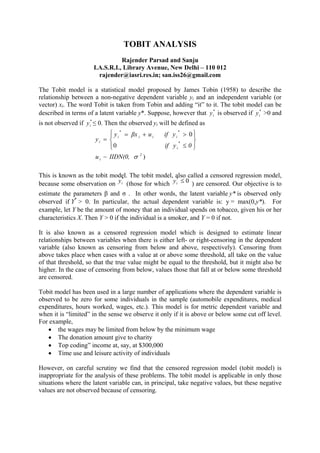
1.
TOBIT ANALYSIS
Rajender Parsad and Sanju
I.A.S.R.I., Library Avenue, New Delhi – 110 012
rajender@iasri.res.in; san.iss26@gmail.com
The Tobit model is a statistical model proposed by James Tobin (1958) to describe the
relationship between a non-negative dependent variable yi and an independent variable (or
vector) xi. The word Tobit is taken from Tobin and adding “it” to it. The tobit model can be
described in terms of a latent variable y*. Suppose, however that *
iy is observed if *
iy >0 and
is not observed if *
iy ≤ 0. Then the observed yi will be defined as
)~
0
0
2
i
*
i
*
iii
*
i
i
IIDN(0,u
0yif
yifuβxy
y












This is known as the tobit model. The tobit model, also called a censored regression model,
because some observation on
*
iy (those for which 0*
iy ) are censored. Our objective is to
estimate the parameters β and σ . In other words, the latent variable y* is observed only
observed if Y*
> 0. In particular, the actual dependent variable is: y = max(0,y*). For
example, let Y be the amount of money that an individual spends on tobacco, given his or her
characteristics X. Then Y > 0 if the individual is a smoker, and Y = 0 if not.
It is also known as a censored regression model which is designed to estimate linear
relationships between variables when there is either left- or right-censoring in the dependent
variable (also known as censoring from below and above, respectively). Censoring from
above takes place when cases with a value at or above some threshold, all take on the value
of that threshold, so that the true value might be equal to the threshold, but it might also be
higher. In the case of censoring from below, values those that fall at or below some threshold
are censored.
Tobit model has been used in a large number of applications where the dependent variable is
observed to be zero for some individuals in the sample (automobile expenditures, medical
expenditures, hours worked, wages, etc.). This model is for metric dependent variable and
when it is “limited” in the sense we observe it only if it is above or below some cut off level.
For example,
 the wages may be limited from below by the minimum wage
 The donation amount give to charity
 Top coding” income at, say, at $300,000
 Time use and leisure activity of individuals
However, on careful scrutiny we find that the censored regression model (tobit model) is
inappropriate for the analysis of these problems. The tobit model is applicable in only those
situations where the latent variable can, in principal, take negative values, but these negative
values are not observed because of censoring.

2. Tobit Analysis
Expenditureonhousing
To explain this model, we have a data on housing expenditure in relation to income for a
cross section of 30 families. Now our interest is in finding out the amount of money a person
or family spends on a house in relation to socioeconomic variables. If a consumer does not
purchase a house, obviously we have no data on housing expenditure for such consumers; we
have such data only on consumers who actually purchase a house.
Thus consumers are divided into two groups, one consisting of, say, n1 consumers amount
whom we have information on the regressors (say, income, number of people in the family,
mortgage interest rate, etc.) as well as the regressand (amount of expenditure on housing) and
another consisting of n2 consumers about whom we have information only on the regressors
but not on the regressand.
We cannot estimate regression using only n1 observations. If we use OLS estimates of the
parameters obtained from the subset of n1 observation will be biased as well as inconsistent;
that is, they are biased even asymptotically. The bias arises from the fact that if we consider
only the n1 observations and omit the others, there is no guarantee that E(ui) will be
necessarily zero and without E(ui)=0 we cannot guarantee that the OLS estimates will be
unbiased.
x: Expenditure data not
available, but income
data available
: Both expenditure and
income data available
Y
x x x x x X
Income
As the figure shows, if Y is not observed (because of censoring), all such observations (= n2),
denoted by crosses, will lie on the horizontal axis. If Y is observed, the observations(= n1),
denoted by dots, will lie in the X-Y plane. If we estimate a regression line based on the n1
observations only, the resulting intercept and slope coefficients are bound to be different than
if all the (n1+n2) observations were taken into account.
There is sometimes confusion about the difference between truncated model and censored
model. With censored variables, all of the observations are in the dataset, but we don't know
the "true" values of some of them. In the censored model we have observation on the

3. Tobit Analysis
explanatory variable ix for all individuals. It is only the dependent variable *
iy that is missing
for some individuals. In the truncated model, we have no data on either *
iy or ix for some
individuals because no samples are drawn if *
iy is below or above a certain level.
To estimate a Tobit model in SAS, we can use either the QLIM procedure of SAS/ETS or the
LIFEREG procedure of SAS/STAT. QLIM represents qualitative and limited dependent
variable. An example of Tobit analysis using QLIM s also given at
http://support.sas.com/documentation/cdl/en/etsug/60372/HTML/default/viewer.htm#etsug_qlim_sect
034.htm
A lots of problems related to this are available in literature. The following is one example
which we have taken from the website http://www.ats.ucla.edu/stat/sas/dae/tobit.htm.
Example 1: Consider the situation in which we have a measure of academic aptitude (scaled
200-800) which we want to model using reading and math test scores, as well as, the type of
program the student is enrolled in (academic, general, or vocational). The students who
answer all questions on the academic aptitude test correctly receive a score of 800, even
though it is likely that these students are not "truly" equal in aptitude. The same is true of
students who answer all of the questions incorrectly. All such students would have a score of
200, although they may not all be of equal aptitude. The problem here is that in the dataset,
the lowest value of academic aptitude is 352. And no students received a score of 200 (i.e. the
lowest score possible), meaning that even though censoring from below was possible, but it
does not occur in the dataset.
Solution:
“Here the academic aptitude variable is denoted by apt, the reading and math test scores are
read and math respectively. The variable prog is the type of program the student is in, it is a
categorical (nominal) variable that takes on three values, academic (prog = 1), general (prog
= 2), and vocational (prog = 3).”
data sastobit;
input id read math prog apt;
format prog pro.;
cards;
1 34 40 3 352
2 39 33 3 449
3 63 48 2 648
4 44 41 2 501
5 47 43 2 762
6 47 46 2 658
7 57 59 2 800
8 39 52 2 613
9 48 52 3 531
10 47 49 1 528
11 34 45 2 584
12 37 45 3 610
13 47 39 3 586
14 47 54 2 769
15 39 44 3 402

4. Tobit Analysis
16 47 44 3 521
17 47 48 2 478
18 50 49 3 629
19 28 43 1 603
20 60 57 2 633
21 44 61 1 724
22 42 39 3 515
23 65 64 2 748
24 52 66 2 634
25 47 42 1 630
26 60 62 2 800
27 53 61 2 652
28 39 54 1 621
29 52 49 1 683
30 41 42 2 531
31 55 52 1 625
32 50 66 3 605
33 57 72 2 698
34 73 57 2 679
35 60 50 1 691
36 44 44 1 612
37 41 40 3 572
38 45 50 2 625
39 66 67 2 734
40 42 43 1 551
41 50 45 2 549
42 46 55 3 622
43 47 43 2 557
44 47 45 3 678
45 34 41 3 467
46 45 44 2 631
47 47 49 2 625
48 57 52 2 584
49 50 39 3 485
50 50 42 1 568
51 42 42 1 593
52 50 53 2 590
53 34 46 3 529
54 47 46 1 661
55 52 49 2 579
56 55 46 3 502
57 71 72 2 794
58 55 40 3 529
59 65 63 2 703
60 57 51 2 635
61 76 60 2 765
62 65 48 1 732
63 52 60 1 537
64 50 45 3 648
65 55 66 2 667

5. Tobit Analysis
66 68 56 3 576
67 37 42 3 476
68 73 71 2 797
69 44 40 3 548
70 57 41 1 599
71 57 56 1 766
72 42 47 3 596
73 50 53 2 716
74 57 50 2 661
75 60 51 3 548
76 47 51 2 595
77 61 49 2 689
78 39 54 2 577
79 60 49 2 633
80 65 68 2 713
81 63 59 2 668
82 68 65 2 800
83 50 41 3 571
84 63 54 1 636
85 55 57 1 691
86 44 54 1 682
87 50 46 1 605
88 68 64 2 618
89 35 40 3 522
90 42 50 2 671
91 50 56 3 666
92 52 57 1 739
93 73 62 2 800
94 55 61 2 782
95 73 71 2 800
96 65 61 2 749
97 60 58 2 613
98 57 51 3 648
99 47 56 1 640
100 63 71 2 793
101 60 67 2 800
102 52 51 2 698
103 76 64 2 676
104 54 57 2 630
105 50 45 2 598
106 36 37 3 404
107 47 47 3 629
108 34 41 1 637
109 42 42 1 574
110 52 50 3 620
111 39 39 1 622
112 52 48 2 689
113 44 51 2 556
114 68 62 2 725
115 42 43 1 571

6. Tobit Analysis
116 57 54 2 681
117 34 39 3 565
118 55 58 1 629
119 42 45 1 584
120 63 54 2 589
121 68 53 3 788
122 52 58 2 779
123 68 56 1 605
124 42 41 3 614
125 68 58 2 768
126 42 57 1 715
127 63 57 2 770
128 39 38 2 508
129 44 46 1 527
130 43 55 1 685
131 65 57 2 649
132 73 73 2 800
133 50 40 3 535
134 44 39 1 474
135 63 65 2 696
136 65 70 2 792
137 63 65 2 800
138 43 40 3 427
139 68 61 2 800
140 44 40 3 399
141 63 47 3 566
142 47 52 3 523
143 63 75 3 800
144 60 58 1 712
145 42 38 3 458
146 55 64 2 688
147 47 53 2 619
148 42 51 3 565
149 63 49 1 727
150 42 57 3 554
151 47 52 3 633
152 55 56 2 687
153 39 40 3 665
154 65 66 2 796
155 44 46 1 614
156 50 53 2 618
157 68 58 1 733
158 52 55 1 657
159 55 54 2 592
160 55 55 2 746
161 57 72 2 800
162 57 40 3 702
163 52 64 2 800
164 31 46 3 516
165 36 54 3 604

7. Tobit Analysis
166 52 53 2 669
167 63 35 1 563
168 52 57 2 695
169 55 63 1 779
170 47 61 2 712
171 60 60 2 678
172 47 57 2 618
173 50 61 1 650
174 68 71 2 750
175 36 42 1 454
176 47 41 2 586
177 55 62 2 688
178 47 57 3 640
179 47 60 2 609
180 71 69 2 800
181 50 45 2 662
182 44 43 2 462
183 63 49 2 591
184 50 53 3 496
185 63 55 2 647
186 57 63 2 681
187 57 57 1 800
188 63 56 2 796
189 47 63 2 669
190 47 54 2 661
191 47 43 2 567
192 65 63 2 800
193 44 48 2 666
194 63 69 2 800
195 57 60 1 727
196 44 49 2 539
197 50 50 2 594
198 47 51 2 616
199 52 50 2 558
200 68 75 2 800
;
proc print data=sastobit;
run;
Variable prog comes with a format provided below.
proc format ;
value prog 1="academic"
2="general"
3="vocational";
run;
To obtain the summary statistics for apt, read and math for each of the three programmes
separately, use the following statements

8. Tobit Analysis
proc means data = sastobit maxdec=2 nonobs;
class prog;
vars apt read math;
run;
The results are given in Table 1.1.
Table 1.1
prog Variable N Mean
Std
Dev Minimum Maximum
academic apt
read
math
45
45
45
639.02
49.76
50.02
78.63
9.23
7.44
454.00
28.00
35.00
800.00
68.00
63.00
general apt
read
math
105
105
105
677.76
56.16
56.73
88.21
9.59
8.73
462.00
34.00
38.00
800.00
76.00
75.00
vocational apt
read
math
50
50
50
561.72
46.20
46.42
92.76
8.91
7.95
352.00
31.00
33.00
800.00
68.00
75.00
For depicting the distribution of apt in Histogram, use the following statements
proc sgplot data = sastobit noautolegend;
histogram apt;
density apt /type = normal lineattrs=(color=blue);
run;
The results are presented in Figure 1.1.
Figure 1.1
Looking at the above histogram showing the distribution of apt, we can see the censoring in
the data, that is, there are far more cases with scores of 775 to 800 than one would expect
looking at the rest of the distribution. Further, fit a normal distribution to the apt data using
the following statememts:
proc univariate data=sastobit noprint;
histogram apt / midpoints=350 to 800 by 1 normal ;
run;

9. Tobit Analysis
The results are presented in Tables 2.1 and 2.2 and Figure 2.1
Table 2.1
Table 2.2
Goodness-of-Fit Tests for Normal Distribution
Test Statistic p Value
Kolmogorov-
Smirnov
D 0.056072
62
Pr > D 0.126
Cramer-von
Mises
W-Sq 0.079552
20
Pr > W-Sq 0.216
Anderson-
Darling
A-Sq 0.935990
49
Pr > A-Sq 0.019
At the α = 0.05 significance level, kolmogorov-Smirnov and Cramer-von Mises tests support
the conclusion that the normal distribution with mean μ= 640.035, and standards deviation σ
=99.21903 provides a good model for the distribution of academic aptitude.
Figure 2.1
In the histogram above, midpoints option is used to produce a histogram where each unique
value of apt has its own bar by specifying that there should be bins from 350 (the minimum
of apt is 352) and a max of 800 in units of 1. The spike on the far right of the histogram is the
bar for cases where apt=800, the height of this bar relative to all the others clearly shows the
excess number of cases with this value. To study the correlation between read, math and apt,
one can use the following statements and the results are given in Table 3.1 and Figure 3.1.
ods graphics on;
proc corr data = sastobit nosimple;
var read math apt;
run;
ods graphics off;
Parameters for Normal
Distribution
Parameter Symbol Estimate
Mean Mu 640.035
Std Dev Sigma 99.21903

10. Tobit Analysis
Table 3.1
Pearson Correlation Coefficients, N = 200
Prob > |r| under H0: Rho=0
read math apt
read 1.00000 0.66228
<.0001
0.64512
<.0001
math 0.66228
<.0001
1.00000 0.73327
<.0001
apt 0.64512
<.0001
0.73327
<.0001
1.00000
Figure 3.1
The collection of cases at the top of the bottom row of the scatter plots are due to the
censoring in the distribution of apt. The QLIM Procedure
proc qlim data = sastobit ;
class prog;
model apt = read math prog;
endogenous apt ~ censored (ub=800);
run;
In the above, the class statement identifies prog (represented as programme in which the
students get enrolled) as a categorical variable. Here “1” denotes acdemic program, “2”
denotes general program and “3” denotes vocational program. The model statement specifies
that apt should be modeled using read, math, and prog. The endogenous statement specifies
that the outcome variable apt is censored, with an upper bound of 800 (i.e. ub=800). The
results are given in Tables 4.1, 4.2, 4.3 and 4.4.

11. Tobit Analysis
Table 4.1
Summary Statistics of Continuous Responses
Variable Mean
Standard
Error Type
Lower
Bound
Upper
Bound
N Obs
Lower
Bound
N Obs
Upper
Bound
apt 640.035 99.219030 Censored 800 17
Above table 4.1 provides a summary of the number of left- and right-censored values.
Table 4.2
Class Level Information
Class Levels Values
prog 3 academic general vocational
The class level information shows that prog is a classification variable taking values 1, 2 and
3.
Table 4.3
Model Fit Summary
Number of Endogenous Variables 1
Endogenous Variable apt
Number of Observations 200
Log Likelihood -1041
Maximum Absolute Gradient 8.40561E-7
Number of Iterations 26
Optimization Method Quasi-Newton
AIC 2094
Schwarz Criterion 2114
Table 4.3 labelled Model Fit Summary includes information on the number of observations
(200), the number of iterations it took the model to converge, the final log likelihood, and the
AIC and Schwarz Criterion (also known as the BIC).

12. Tobit Analysis
Table 4.4
Parameter Estimates
Parameter DF Estimate
Standard
Error
t Val
ue
Approx
Pr > |t|
Intercept 1 163.422155 30.408580 5.37 <.0001
read 1 2.697939 0.618806 4.36 <.0001
math 1 5.914484 0.709818 8.33 <.0001
prog academic 1 46.143900 13.724195 3.36 0.0008
prog general 1 33.429162 12.955628 2.58 0.0099
prog vocational 0 0 . . .
_Sigma 1 65.676720 3.481423 18.86 <.0001
The coefficients for read and math are statistically significant, as are the terms for
prog="academic" and prog="general" (with prog="vocational" as the reference category).
Tobit regression coefficients are interpreted in the same manner as OLS regression
coefficients. A one unit increase in read is associated with a 2.7 point increase in the
predicted value of apt. A one unit increase in math is associated with a 5.9 point increase in
the predicted value of apt. The terms for prog have a slightly different interpretation. The
predicted value of apt is 46.14 higher for students in an academic program
(prog="academic") than for students in a vocational program (prog="vocational"). The
predicted value of apt is 33.43 points higher for students in a general program
(prog="general") than for students in a vocational program (prog="vocational").
In the “Parameter Estimates” table there are seven rows. The first six of these rows
correspond to the vector estimate of the regression coefficients . The last one is called
_Sigma, which corresponds to the estimate of the error variance σ .
We can include a test of the overall effect of prog, by testing whether the coefficients for
prog="academic" and prog="general" are simultaneously equal to 0. To do this we add a test
statement to the proc qlim code. To figure out how SAS names the dummy variables for a
class variable, it is usually a good idea to output the parameter estimates as a data set (in this
example, we named it as t) and print it out to see how internally SAS names these variables.
In our example, we see that SAS has appended the value label to prog in naming the dummy
variables for prog. The results obtained are given in Tables 5.1 and 5.2.
proc qlim data = sastobit outest=t;
class prog;
model apt = read math prog;
endogenous apt ~ censored (ub=800);
run;
proc print data = t noobs;
run;

13. Tobit Analysis
Table 5.1
_NAME_ _TYPE_ _STATUS_ Intercept read math
Progacad
emic
Progge
neral
Progvo
catinal _Sigma
PARM 0 Converged 163.422 2.69794 5.91448 46.1439 33.4292 . 65.6767
STD 0 Converged 30.409 0.61881 0.70982 13.7242 12.9556 . 3.4814
proc qlim data =sastobit ;
class prog;
model apt = read math prog;
endogenous apt ~ censored (ub=800);
test 'prog' progacademic = 0,
proggeneral = 0;
run;
Table 5.2
Test Results
Test Type Statistic Pr > ChiSq Label
'prog' Wald 11.96 0.0025 progacademic = 0 , proggeneral = 0
We may also wish to evaluate how well our model fits. This can be particularly useful when
comparing competing models. One method of assessing model fit is to compare the predicted
values based on the tobit model to the observed values in the dataset. Below we use proc qlim
to generate predicted values along with the data via the output statement. Then proc corr is
used to estimate the correlation between the predicted and observed values of apt. The
predicted values are given in Table 6.1.
proc qlim data=sastobit ;
model apt = read math prog;
endogenous apt ~ censored (ub=800);
output out = temp1 predicted;
run;
proc print data=temp1;
run;
Table 6.1
Obs id read math prog apt P_apt
1 1 34 40 3 352 493.356
2 2 39 33 3 449 464.504
3 3 63 48 2 648 645.855
4 4 44 41 2 501 550.096
5 5 47 43 2 762 570.686
6 6 47 46 2 658 589.025
7 7 57 59 2 800 696.371
8 8 39 52 2 613 603.400
9 9 48 52 3 531 605.742
10 10 47 49 1 528 630.112
11 11 34 45 2 584 546.670

14. Tobit Analysis
Obs id read math prog apt P_apt
12 12 37 45 3 610 532.285
13 13 47 39 3 586 523.485
14 14 47 54 2 769 637.929
15 15 39 44 3 402 531.747
16 16 47 44 3 521 554.050
17 17 47 48 2 478 601.251
18 18 50 49 3 629 592.978
19 19 28 43 1 603 540.466
20 20 60 57 2 633 692.509
21 21 44 61 1 724 695.105
22 22 42 39 3 515 509.546
23 23 65 64 2 748 749.239
24 24 52 66 2 634 725.223
25 25 47 42 1 630 587.321
26 26 60 62 2 800 723.074
27 27 53 61 2 652 697.446
28 28 39 54 1 621 638.375
29 29 52 49 1 683 644.051
30 30 41 42 2 531 547.846
31 31 55 52 1 625 670.754
32 32 50 66 3 605 696.899
33 33 57 72 2 698 775.840
34 34 73 57 2 679 728.750
35 35 60 50 1 691 672.467
36 36 44 44 1 612 591.184
37 37 41 40 3 572 512.871
38 38 45 50 2 625 607.901
39 39 66 67 2 734 770.365
40 40 42 43 1 551 579.495
41 41 50 45 2 549 591.275
42 42 46 55 3 622 618.505
43 43 47 43 2 557 570.686
44 44 47 45 3 678 560.163
45 45 34 41 3 467 499.469
46 46 45 44 2 631 571.223
47 47 47 49 2 625 607.364
48 48 57 52 2 584 653.580
49 49 50 39 3 485 531.848
50 50 50 42 1 568 595.685
51 51 42 42 1 593 573.382
52 52 50 53 2 590 640.179
53 53 34 46 3 529 530.034
54 54 47 46 1 661 611.773
55 55 52 49 2 579 621.303
56 56 55 46 3 502 588.578
57 57 71 72 2 794 800.000
58 58 55 40 3 529 551.900

15. Tobit Analysis
Obs id read math prog apt P_apt
59 59 65 63 2 703 743.126
60 60 57 51 2 635 647.467
61 61 76 60 2 765 755.452
62 62 65 48 1 732 674.180
63 63 52 60 1 537 711.294
64 64 50 45 3 648 568.526
65 65 55 66 2 667 733.587
66 66 68 56 3 576 685.949
67 67 37 42 3 476 513.946
68 68 73 71 2 797 800.000
69 69 44 40 3 548 521.234
70 70 57 41 1 599 609.086
71 71 57 56 1 766 700.781
72 72 42 47 3 596 558.450
73 73 50 53 2 716 640.179
74 74 57 50 2 661 641.354
75 75 60 51 3 548 633.082
76 76 47 51 2 595 619.590
77 77 61 49 2 689 646.393
78 78 39 54 2 577 615.626
79 79 60 49 2 633 643.605
80 80 65 68 2 713 773.691
81 81 63 59 2 668 713.098
82 82 68 65 2 800 763.715
83 83 50 41 3 571 544.074
84 84 63 54 1 636 705.282
85 85 55 57 1 691 701.319
86 86 44 54 1 682 652.314
87 87 50 46 1 605 620.137
88 88 68 64 2 618 757.602
89 89 35 40 3 522 496.144
90 90 42 50 2 671 599.538
91 91 50 56 3 666 635.769
92 92 52 57 1 739 692.955
93 93 73 62 2 800 759.315
94 94 55 61 2 782 703.022
95 95 73 71 2 800 800.000
96 96 65 61 2 749 730.900
97 97 60 58 2 613 698.622
98 98 57 51 3 648 624.719
99 99 47 56 1 640 672.903
100 100 63 71 2 793 786.454
101 101 60 67 2 800 753.639
102 102 52 51 2 698 633.528
103 103 76 64 2 676 779.904
104 104 54 57 2 630 675.782
105 105 50 45 2 598 591.275

16. Tobit Analysis
Obs id read math prog apt P_apt
106 106 36 37 3 404 480.593
107 107 47 47 3 629 572.389
108 108 34 41 1 637 544.967
109 109 42 42 1 574 573.382
110 110 52 50 3 620 604.667
111 111 39 39 1 622 546.680
112 112 52 48 2 689 615.190
113 113 44 51 2 556 611.226
114 114 68 62 2 725 745.376
115 115 42 43 1 571 579.495
116 116 57 54 2 681 665.806
117 117 34 39 3 565 487.243
118 118 55 58 1 629 707.432
119 119 42 45 1 584 591.721
120 120 63 54 2 589 682.533
121 121 68 53 3 788 667.610
122 122 52 58 2 779 676.319
123 123 68 56 1 605 731.447
124 124 42 41 3 614 521.772
125 125 68 58 2 768 720.924
126 126 42 57 1 715 665.077
127 127 63 57 2 770 700.872
128 128 39 38 2 508 517.818
129 129 44 46 1 527 603.410
130 130 43 55 1 685 655.639
131 131 65 57 2 649 706.448
132 132 73 73 2 800 800.000
133 133 50 40 3 535 537.961
134 134 44 39 1 474 560.619
135 135 63 65 2 696 749.776
136 136 65 70 2 792 785.917
137 137 63 65 2 800 749.776
138 138 43 40 3 427 518.447
139 139 68 61 2 800 739.263
140 140 44 40 3 399 521.234
141 141 63 47 3 566 616.993
142 142 47 52 3 523 602.954
143 143 63 75 3 800 788.157
144 144 60 58 1 712 721.371
145 145 42 38 3 458 503.433
146 146 55 64 2 688 721.361
147 147 47 53 2 619 631.816
148 148 42 51 3 565 582.902
149 149 63 49 1 727 674.717
150 150 42 57 3 554 619.580
151 151 47 52 3 633 602.954
152 152 55 56 2 687 672.457

17. Tobit Analysis
Obs id read math prog apt P_apt
153 153 39 40 3 665 507.295
154 154 65 66 2 796 761.465
155 155 44 46 1 614 603.410
156 156 50 53 2 618 640.179
157 157 68 58 1 733 743.673
158 158 52 55 1 657 680.729
159 159 55 54 2 592 660.231
160 160 55 55 2 746 666.344
161 161 57 72 2 800 775.840
162 162 57 40 3 702 557.476
163 163 52 64 2 800 712.997
164 164 31 46 3 516 521.671
165 165 36 54 3 604 584.514
166 166 52 53 2 669 645.754
167 167 63 35 1 563 589.135
168 168 52 57 2 695 670.206
169 169 55 63 1 779 737.997
170 170 47 61 2 712 680.719
171 171 60 60 2 678 710.848
172 172 47 57 2 618 656.268
173 173 50 61 1 650 711.832
174 174 68 71 2 750 800.000
175 175 36 42 1 454 556.656
176 176 47 41 2 586 558.460
177 177 55 62 2 688 709.135
178 178 47 57 3 640 633.519
179 179 47 60 2 609 674.607
180 180 71 69 2 800 796.530
181 181 50 45 2 662 591.275
182 182 44 43 2 462 562.322
183 183 63 49 2 591 651.968
184 184 50 53 3 496 617.430
185 185 63 55 2 647 688.646
186 186 57 63 2 681 720.823
187 187 57 57 1 800 706.894
188 188 63 56 2 796 694.759
189 189 47 63 2 669 692.945
190 190 47 54 2 661 637.929
191 191 47 43 2 567 570.686
192 192 65 63 2 800 743.126
193 193 44 48 2 666 592.887
194 194 63 69 2 800 774.228
195 195 57 60 1 727 725.233
196 196 44 49 2 539 599.000
197 197 50 50 2 594 621.840
198 198 47 51 2 616 619.590

18. Tobit Analysis
Obs id read math prog apt P_apt
199 199 52 50 2 558 627.416
200 200 68 75 2 800 800.000
proc corr data = temp1 nosimple;
var apt p_apt;
run;
The correlation between observed and predicted values is given in Table 6.2 and scatter plot
in Figure 6.1.
Pearson Correlation Coefficients, N = 200
Prob > |r| under H0: Rho=0
Table 6.2
Figure 6.1
The output from proc corr gives the correlation between the predicted and observed values of
apt, which is 0.78094. If we square this value, we get the squared multiple correlation, this
indicates that the predicted values share about 61% (0.78094^2 = .6099) of their variance
with the observed values of apt.
apt P_apt
apt 1.00000 0.78094
<0.0001
P_apt 0.78094
<.0001
1.00000

19. Tobit Analysis
Some Important Points
Below is a list of some analysis methods you may have encountered. Some of the methods
listed are quite reasonable while others have either fallen out of favor or have limitations.
One can analyze these data using OLS regression. OLS regression will treat the 800 as the
actual values and not as the upper limit of the top academic aptitude. A limitation of this
approach is that when the variable is censored, OLS provides inconsistent estimates of the
parameters, meaning that the coefficients from the analysis will not necessarily approach the
"true" population parameters as the sample size increases.
There is sometimes confusion about the difference between truncated data and censored data.
With censored variables, all of the observations are in the dataset, but we don't know the
"true" values of some of them. With truncation some of the observations are not included in
the analysis because of the value of the variable. When a variable is censored, regression
models for truncated data provide inconsistent estimates of the parameters.
References:
SAS Data Analysis Examples Tobit Analysis at
http://www.ats.ucla.edu/stat/sas/dae/tobit.htm
Robin, James (1958), "Estimation of relationships for limited dependent
variables", Econometrica (The Econometric Society) 26 (1): 24–36, doi:10.2307/190738
http://en.wikipedia.org/wiki/Tobit_model
http://www.ats.ucla.edu/stat/stata/dae/tobit.htm
http://support.sas.com/documentation/cdl/en/etsug/60372/HTML/default/viewer.htm#etsug_q
lim_sect034.htm