
Recommended
More Related Content
Similar to Lecture30
Similar to Lecture30 (12)
More from zukun
More from zukun (20)
Recently uploaded
Recently uploaded (20)
Lecture30
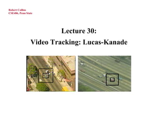
- 1. Robert Collins CSE486, Penn State Lecture 30: Video Tracking: Lucas-Kanade
- 2. Robert Collins CSE486, Penn State Two Popular Tracking Methods • Mean-shift color histogram tracking (last time) • Lucas-Kanade template tracking (today)
- 3. Robert Collins CSE486, Penn State Lucas-Kanade Tracking
- 4. Robert Collins CSE486, Penn State Review: Lucas-Kanade • Brightness constancy • One equation two unknowns unknown flow vector temporal gradient spatial gradient • How to get more equations for a pixel? – Basic idea: impose additional constraints • one method: pretend the pixel’s neighbors have the same (u,v) – If we use a 5x5 window, that gives us 25 equations per pixel! * From Khurram Hassan-Shafique CAP5415 Computer Vision 2003
- 5. Robert Collins CSE486, Penn State Review: Lucas-Kanade (cont) • Now we have more equations than unknowns • Solution: solve least squares problem – minimum least squares solution given by solution (in d) of: – The summations are over all pixels in the K x K window – This technique was first proposed by Lucas & Kanade (1981) • described in Trucco & Verri reading * From Khurram Hassan-Shafique CAP5415 Computer Vision 2003
- 6. Robert Collins CSE486, Penn State Lucas Kanade Tracking Traditional Lucas-Kanade is typically run on small, corner-like features (e.g. 5x5) to compute optic flow. Observation: There’s no reason we can’t use the same approach on a larger window around the object being tracked. 80x50 pixels
- 7. Robert Collins Basic LK Derivation for Templates CSE486, Penn State template (model) current frame u,v = hypothesized location of template in current frame
- 8. Robert Collins Basic LK Derivation for Templates CSE486, Penn State First order approx Take partial derivs and set to zero Form matrix equation solve via least-squares
- 9. Robert Collins CSE486, Penn State One Problem with this... Assumption of constant flow (pure translation) for all pixels in a larger window is unreasonable for long periods of time. However, we can easily generalize Lucas-Kanade approach to other 2D parametric motion models (like affine or projective) by introducing a “warp” function W. generalize x [ I (W ([ x, y ]; P)) T ([ x, y ])]2 within image patch y
- 10. Robert Collins CSE486, Penn State Step-by-Step Derivation The key to the derivation is Taylor series approximation: W [ I (W ([ x, y ]; P P)) ~ [ I (W ([ x, y ]; P)) I ~ P P We will derive this step-by-step. First, we need two background formula:
- 11. Robert Collins CSE486, Penn State Step-by-Step Derivation First consider the expansion for a single variable p
- 12. Robert Collins CSE486, Penn State Step-by-Step Derivation Note that each variable parameter pi contributes a term of the form
- 13. Robert Collins CSE486, Penn State Step-by-Step Derivation Now let’s rewrite the expression as a matrix equation. For each term, we can rewrite: So that we have:
- 14. Robert Collins CSE486, Penn State Step-by-Step Derivation Further collecting the dw/dpi terms into a matrix, we can write: which are the terms in the matrix equation: ~ W [ I (W ([ x, y ]; P P)) ~ [ I (W ([ x, y ]; P)) I P P
- 15. Robert Collins Example: Jacobian of Affine Warp CSE486, Penn State Let W([x, y]; P) [Wx , Wy ] general equation of Jacobian Wx Wx Wx Wx W P P P P 1 2 3 n P Wy Wy Wy Wy P 1 P2 P3 P n affine warp function (6 parameters) x xP yP3 P5 1 x W xP2 y yP4 P6 1 p1 W ([ x, y ]; P ) p3 p5 y p6 P P p2 1 p4 1 x 0 y 0 1 0 0 x 0 y 0 1
- 16. Source: “Lucas-Kanade 20 years on: A unifying framework” Baker and Mathews, IJCV 04 Robert Collins CSE486, Penn State Iterate Warp I to obtain I(W([x y];P)) Compute the error image T(x) – I(W([x y]; P)) Warp the gradient I with W([x y]; P) W Evaluate at ([x y]; P) (Jacobian) P W Compute steepest descent images I P W T W Compute Hessian matrix (I P ) (I P ) W T Compute ( I P ) (T ( x, y ) I (W ([ x, y ]; P ))) Compute P Update P P + P Until P magnitude is negligible Dr. Ng Teck Khim
- 17. Robert Collins CSE486, Penn State Algorithm At a Glance Source: “Lucas-Kanade 20 years on: A unifying framework” Baker and Mathews, IJCV 04
- 18. Robert Collins State of the Art Lucas Kanade Tracking CSE486, Penn State Tracking facial mesh models (piecewise affine) QuickTime™ and a YUV420 codec decompressor are needed to see this picture. Baker, Matthews, CMU