PCM Waveforms Spectral densities of PCM waveforms Multi Level Signaling Demodulation/Detection

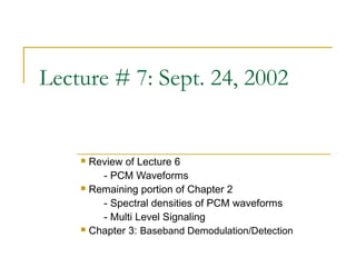
1. Lecture # 7: Sept. 24, 2002
 Review of Lecture 6
- PCM Waveforms
 Remaining portion of Chapter 2
- Spectral densities of PCM waveforms
- Multi Level Signaling
 Chapter 3: Baseband Demodulation/Detection

2. Generation of Line Codes
 The FIR filter realizes the different pulse shapes
 Baseband modulation with arbitrary pulse shapes can be detected
by
 correlation detector
 matched filter detector (this is the most common detector)

3. Comparisons of Line Codes
 Different pulse shapes are used
 to control the spectrum of the transmitted signal (no DC value,
bandwidth, etc.)
 guarantee transitions every symbol interval to assist in symbol timing
recovery
1. Power Spectral Density of Line Codes (see Fig. 2.23, Page 90)
 After line coding, the pulses may be filtered or shaped to further
improve there properties such as
 Spectral efficiency
 Immunity to Intersymbol Interference
 Distinction between Line Coding and Pulse Shaping is not easy
2. DC Component and Bandwidth
 DC Components
 Unipolar NRZ, polar NRZ, and unipolar RZ all have DC components
 Bipolar RZ and Manchester NRZ do not have DC components

4.  First Null Bandwidth
 Unipolar NRZ, polar NRZ, and bipolar all have 1st null bandwidths of
Rb = 1/Tb
 Unipolar RZ has 1st null BW of 2Rb
 Manchester NRZ also has 1st null BW of 2Rb, although the
spectrum becomes very low at 1.6Rb

5.  Section 2.8.4: Bits per PCM Word and Bits per Symbol
 L=2l
 Section 2.8.5: M-ary Pulse Modulation Waveforms
 M = 2k
 Problem 2.14: The information in an analog waveform, whose
maximum frequency fm=4000Hz, is to be transmitted using a 16-level
PAM system. The quantization must not exceed ±1% of the peak-to-
peak analog signal.
(a) What is the minimum number of bits per sample or bits per PCM
word that should be used in this system?
(b) What is the minimum required sampling rate, and what is the
resulting bit rate?
(c) What is the 16-ary PAM symbol Transmission rate?

7. Chapter 3: Baseband
Demodulation/Detection
 Detection of Binary Signal in Gaussian Noise
 Matched Filters and Correlators
 Bayes’ Decision Criterion
 Maximum Likelihood Detector
 Error Performance

8. Demodulation and Detection
AWGN
DETECT
DEMODULATE & SAMPLE
SAMPLE
at t = T
RECEIVED
WAVEFORM FREQUENCY
RECEIVING EQUALIZING
DOWN
FILTER FILTER THRESHOLD MESSAGE
TRANSMITTED CONVERSION
WAVEFORM COMPARISON SYMBOL
OR
CHANNEL
FOR COMPENSATION
SYMBOL
BANDPASS FOR CHANNEL
SIGNALS INDUCED ISI
OPTIONAL
ESSENTIAL
Figure 3.1: Two basic steps in the demodulation/detection of digital signals
The digital receiver performs two basic functions:
 Demodulation, to recover a waveform to be sampled at t = nT.
 Detection, decision-making process of selecting possible digital symbol

9. Detection of Binary Signal in Gaussian
Noise
2
1
0
-1
-2
0 2 4 6 8 10 12 14 16 18 20
2
1
0
-1
-2
0 2 4 6 8 10 12 14 16 18 20
2
1
0
-1
-2
0 2 4 6 8 10 12 14 16 18 20

10. Detection of Binary Signal in Gaussian
Noise
 For any binary channel, the transmitted signal over a symbol interval
(0,T) is:
s0 (t ) 0 ≤ t ≤ T for a binary 0
si (t ) = 
 s1 (t ) 0 ≤ t ≤ T for a binary 1
 The received signal r(t) degraded by noise n(t) and possibly
degraded by the impulse response of the channel hc(t), is
r (t ) = si (t ) * hc (t ) + n(t ) i = 1,2 (3.1)
Where n(t) is assumed to be zero mean AWGN process
 For ideal distortionless channel where hc(t) is an impulse function
and convolution with hc(t) produces no degradation, r(t) can be
represented as:
r (t ) = si (t ) + n(t ) i = 1,2 0≤t ≤T (3.2)

11. Detection of Binary Signal in Gaussian
Noise
 The recovery of signal at the receiver consist of two parts
 Filter
 Reduces the received signal to a single variable z(T)
 z(T) is called the test statistics
 Detector (or decision circuit)
 Compares the z(T) to some threshold level γ0 , i.e.,
H1
z(T ) >
<
γ0 where H1 and H0 are the two
possible binary hypothesis
H0

12. Receiver Functionality
The recovery of signal at the receiver consist of two parts:
1. Waveform-to-sample transformation
 Demodulator followed by a sampler
 At the end of each symbol duration T, predetection point yields a
sample z(T), called test statistic
z (T ) = a (t ) + n (t ) i = 1,2
i 0
(3.3)
Where ai(T) is the desired signal component,
and no(T) is the noise component
1. Detection of symbol
 Assume that input noise is a Gaussian random process and
receiving filter is linear
1  1n 
2

p (n0 ) = exp −  0
 
 
(3.4)
σ 0 2π  2  σ0
  


13.  Then output is another Gaussian random process
1  1  z − a 2 
p ( z | s0 ) = exp  − 
 σ  
0

σ 0 2π  2 0  
 
1  1  z − a 2 
p ( z | s1 ) = exp  − 
 σ  
1

σ 0 2π  2 0  
 
Where σ0 2 is the noise variance
 The ratio of instantaneous signal power to average noise power ,
(S/N)T, at a time t=T, out of the sampler is:
S  ai2
  = 2
 N T σ0 (3.45)
 Need to achieve maximum (S/N)T

14. Find Filter Transfer Function H0(f)
 Objective: To maximizes (S/N)T
 Expressing signal ai(t) at filter output in terms of filter transfer
function H(f)
∞
ai (t ) = ∫ H ( f ) S ( f ) e j 2πft df (3.46)
−∞
where S(f) is the Fourier transform of input signal s(t)
 Output noise power can be expressed as:
N0 ∞
σ = ∫
2
0 | H ( f ) |2 df
2 −∞
(3.47)
 Expressing (S/N)T as:
∞ 2
∫
j 2πfT
H ( f ) S( f ) e df
S  −∞
  =
 N T N0 ∞
2 ∫
−∞
| H ( f ) |2 df (3.48)

15.  For H(f) = H0(f) to maximize (S/N)T, ; use Schwarz’s Inequality:
∞ 2 ∞ 2 ∞ 2
∫ −∞
f1 ( x) f 2 ( x)dx ≤ ∫
−∞
f1 ( x) dx ∫ −∞
f 2 ( x) dx (3.49)
 Equality holds if f1(x) = k f*2(x) where k is arbitrary constant and *
indicates complex conjugate
 Associate H(f) with f1(x) and S(f) ej2π fT with f2(x) to get:
∞ 2 ∞ 2 ∞ 2
∫−∞
H ( f ) S ( f ) e j 2πfT df ≤ ∫ H ( f ) df
−∞ ∫−∞
S ( f ) df (3.50)
 Substitute in eq-3.48 to yield:
S 2 ∞ 2
  ≤
 N T N 0
∫−∞
S ( f ) df
(3.51)

16. S  2E
 Or max   ≤ and energy E of the input signal s(t):
 N T N0
∞ 2
 Thus (S/N)T depends on input signal energy E =∫ S ( f ) df
−∞
and power spectral density of noise and
NOT on the particular shape of the waveform
S 2E
 Equality for max   ≤ holds for optimum filter transfer
 N T N 0
function H0(f)
such that:
H ( f ) = H 0 ( f ) = kS * ( f ) e − j 2πfT (3.54)
h(t ) = ℑ 1 {kS * ( f )e − j 2πfT }
−
(3.55)
 For real valued s(t):  kS (T − t ) 0 ≤ t ≤ T
h(t ) = 
(3.56)
0 else where

17.  The impulse response of a filter producing maximum output signal-
to-noise ratio is the mirror image of message signal s(t), delayed by
symbol time duration T.
 The filter designed is called a MATCHED FILTER
 kS (T − t ) 0 ≤ t ≤ T
h(t ) = 
0 else where
 Defined as:
a linear filter designed to provide the maximum
signal-to-noise power ratio at its output for a given
transmitted symbol waveform

18. Correlation realization of Matched filter
 A filter that is matched to the waveform s(t), has an impulse
response  kS (T − t ) 0 ≤ t ≤T
h(t ) = 
0 else where
 h(t) is a delayed version of the mirror image (rotated on the t = 0
axis) of the original signal waveform
Signal Waveform Mirror image of signal Impulse response of
waveform matched filter
Figure 3.7

19.  This is a causal system
 Recall that a system is causal if before an excitation is applied at
time t = T, the response is zero for - ∝ < t < T
 The signal waveform at the output of the matched filter is
t (3.57)
z (t ) = r (t ) * h(t ) = ∫ r (τ )h(t −τ )dτ
0
 Substituting h(t) to yield:
r (τ ) s[T − (t −τ )]dτ
t
z (t ) = ∫0
r (τ ) s[T − t +τ ]dτ
t
= ∫0 (3.58)
 When t=T,
T
z (t ) = ∫0
r (τ ) s (τ ) dτ
(3.59)

20.  The function of the correlator and matched filter are the same
 Compare (a) and (b)
 From (a)
T
z (t ) = ∫ r (t ) s (t ) dt
0
T
z (t ) t =T = z (T ) = ∫ r (τ ) s (τ )dτ
0

21. From (b) ∞ t
z ' (T ) = r (t ) * h(t ) = ∫ r (τ )h(t − τ )dτ = ∫

r (τ )h(t − τ )dτ
−∞ 0
But
h(t ) = s(T − t ) ⇒ h(t − τ ) = s[T − (t − τ )] = s(T + τ − t )
t
∴ z ' (t ) = ∫ r (τ ) s (τ + T − t )dτ
0
 At the sampling instant t = T, we have
T T
z ' (t ) t −T = z ' (t ) = ∫ r (τ ) s(τ + T − T )dτ = ∫ r (τ ) s (τ )dτ
0 0
 This is the same result obtained in (a)
T
z ' (T ) = ∫ r (τ ) s (τ ) dτ
0
 Hence
z (T ) = z ' (T )